Part A: The Power of Diffusion Models!
Introduction
For project 5a, I opportunity to explore applying noise to images as well as various methods of denoising. I then got then worked with diffusion models to generate samples from a given image as well as a blank noisy canvas. Next I looked into Image-to-image translation for web images as well as hand drawn images. After that I applied inpainting to images given a mask. Finally, I explored visual anagrams and hybrid images.
Part 0. Setup
In part 0, I downloaded a DeepFloyd as well as text embeddings. DeepFloyd is a two stage model trained by Stability AI. Below are a few results with differing numbers of iteratives steps which as a result alter the sample output.
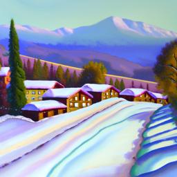
20 iterations

20 iterations
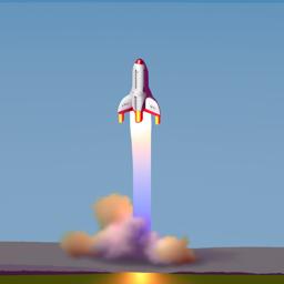
20 iterations

40 iterations
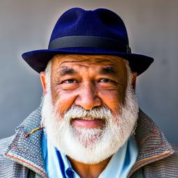
40 iterations

40 iterations
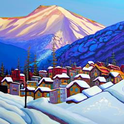
200 iterations
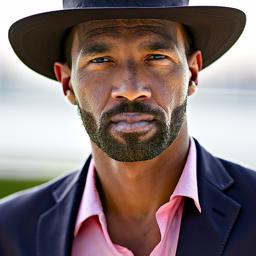
200 iterations
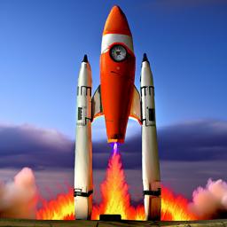
200 iterations
Part 1. Sampling Loops
In this part I wrote my own "sampling loops" that use the pretrained DeepFloyd denoisers. First I implemented the forward process which applied noise to the image. I then implemented various methods of denoising such as classical denoising, one-step denoising, and iterative.
1.1 Implementing the Forward Process
Below I generate a noisy image at timestep t (250,500,750) by sampling from a Gaussian.


1.2 Classical Denoising
Next I applied a Gaussian blur filtering to try to remove the noise from the image. However, the results are not great.


1.3 One-Step Denoising
For this part I use the pretrained diffusion model to denoise the noisy images computed in 1.1. I estimate the noise in the new noisy image and then denoise it using the diffusion model to obtain an estimate of the original image.


1.4 Iterative Denoising
Although the one-step denoising does a decent job for denoising. However, diffusion models are meant to denoise iteratively, but we dont want it to be slow so we can skip steps to denoise faster. To skip steps I created a new list of timesteps called strided_timesteps. I then denoise the image at each timestep in strided_timesteps using the model. Below are the results from every fifth timesteps in strided_timesteps. As well as the final clean image, the original campanile, one-step, and the gaussian blur denoised images.


1.5 Diffusion Model Sampling
Next we use the diffusion model to create images from scratch by passing in a blank canvas with the prompt "a high quality photo" for the embeddings.


1.6 Classifier-Free Guidance (CFG)
From section 1.5, we can see that some of the images in the prior section are not very good, and some are completely non-sensical. In order to improve these results we can use classifier-free guidance. I computed a conditional and an unconditional noise estimate to generate a new estimate using a variable that controls the strength of CFG. For the conditional prompt I used "a high quality photo" and for the unconditional prompt I used "". Below are 5 images using the prompt "a high quality photo" with a CFG scale of 7.


1.7 Image-to-image Translation
The more noise we add, the larger the edit will be however this results in the model needing to hallucinate. I took the original test image, applied the noise function to it, and force it back onto the image manifold without any conditioning. Below I applied this translation to the image of the campanile as well as two images of my own.






1.7.1 Editing Hand-Drawn and Web Images
Next I apply the above function to hand drawn images as well as a image from the web of a porsche. The first image is of an avocado, then I drew a flower and a ball guy with glasses.


1.7.2 Inpainting
Next I applied this function to inpaint an image. This means I took an image, along with a mask, which is used to show what part of the image can be replaced/altered. Then I apply the same function as above to the image while retaining the image outside of the mask. Below are a few examples, the first is changing the top of the campanile, the second is changing the hat of a cartoon boy, and the third is replacing the porsche with a soccer ball. For the first 2 I used the prompt "a high quality image" and for the last I used "a soccer ball" just to try something different.


1.7.3 Text-Conditional Image-to-image Translation
Next I use the same function as above but I guide the projection with a text prompt. I used the prompt "a rocket ship" on various images. I inputted a picture of the iron giant in an attempt to create ironman as well as a picture of a car to create a rocket car. Below are my results.


1.8 Visual Anagrams
Next I applied this functionality to create visual anagrams. In order to do this we pass in two prompts and apply the above functionality with prompt 1 on the original image and then flip the image and apply prompt 2 to it. I then average the two noise estimates to create a new image. Below are a few examples of this and I will attach the prompts as well.


1.9 Hybrid Images
The last part of part A is to use the above function to generate hybrid images, similar to what we did in project 2. In order to create hybrid images compute the noise estimate, by calculating the noise for two different prompts, and then apply a low pass filter on the first image and a high pass filter on the second image. The result would be a hybrid image using the two prompts that we used. Below are a few examples, and I will attach the prompts as well.


Part B: Diffusion Models from Scratch!
Introduction
For part B of this project I trained a UNet model that iteratively denoises an images from the MNIST dataset. I used the algorithms defined in the research paper "Denoising Diffusion Probabilistic Models" by Jonathan Ho, Ajay Jain, and Pieter Abbeel.
Part 1: Training a Single-Step Denoising UNet
1.1 Implementing the UNet
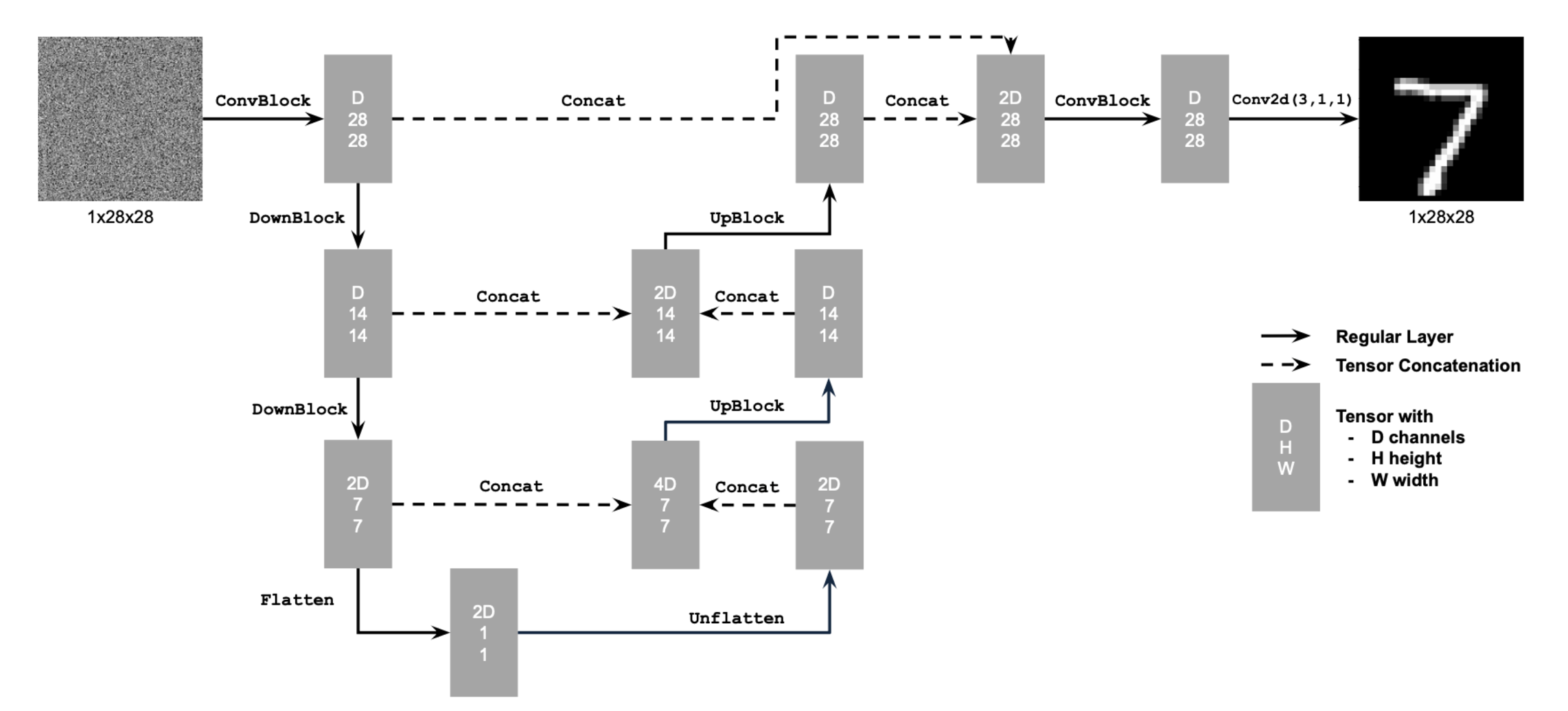
For the first part I built a simple one-step denoiser where I optimized over the L2 loss. The denoiser is implemented as a UNet, which contains downsampling and upsampling blocks with skip connections. Below is the architecture of the UNet.
1.2 Using the UNet to Train a Denoiser
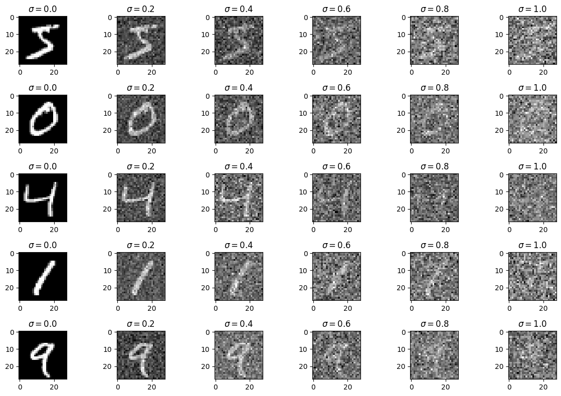
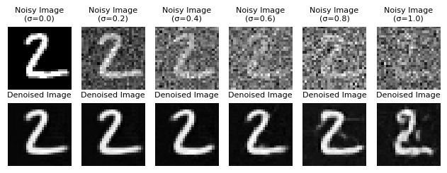
Below is a graph of digits from the MNIST dataset with the noisy function applied at different sigma levels including sigma = [0.0, 0.2, 0.4, 0.6, 0.8. 1.0].
1.3 Training
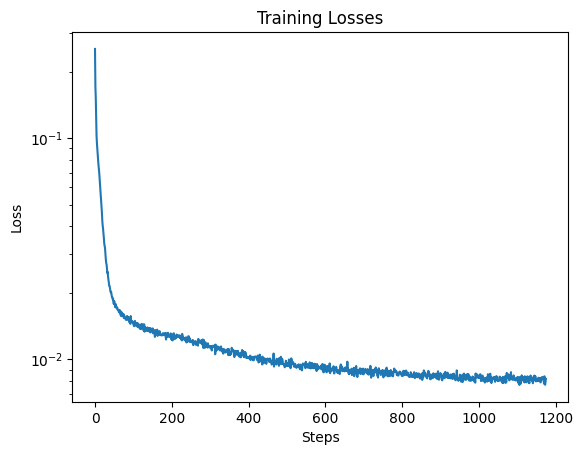
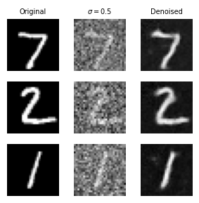
In order to train my model to denoise noisy images, I used sigma = 0.5, and trained for 5 epochs. I used the UNet architecture defined in section 1.1 with a hidden dimension of 128. For the optimizer I used the Adam optimizer with learning rate of 1e-4. Below is a graph of my training loss.
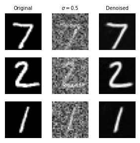
1.4 Out-of-Distribution Testing
The denoiser was trained on sigma = 0.5, so we also want to test how this model performs on images with different noise levels. Below are the results on digits from the test set with varying noise levels.
Part 2: Training a Diffusion Model
2.1 Adding Time Conditioning to UNet
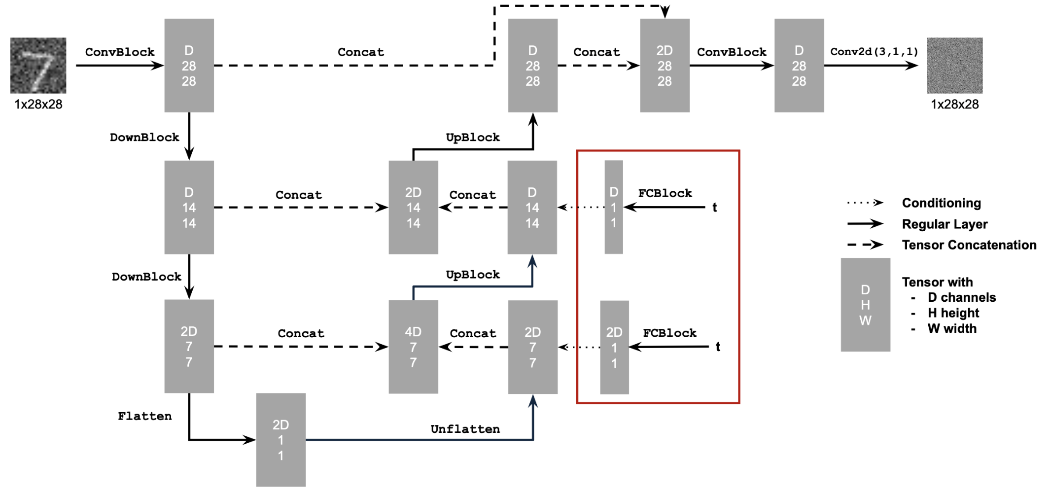
For the next part we transform the uncondtioned UNet into a conditioned UNet on timestep variable t. I injected the scalar t into the UNet model to condition it, and then trained the model to predict a denoised image. Below is the architecture of the conditioned UNet.
2.2 Training the UNet
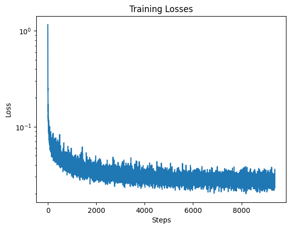
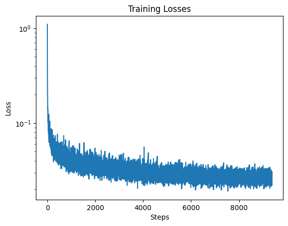
In order to train the model, I pick a random image from the training set, a random timestep t, and train the denoiser to predict the noise. I use the MNIST dataset for the training set with a batch size of 128 and train for 20 epochs. As mentioned in the instructions I normalize t based on T which is the total number of timesteps(300). I used the Adam optimizer with a learning rate of 1e-3. I also call scheduler.step() after every epoch. I used the time-conditioned UNet architecture defined in section 2.1 with a hidden dimension of 64. Below is a graph of my training loss.
2.3 Sampling from the UNet
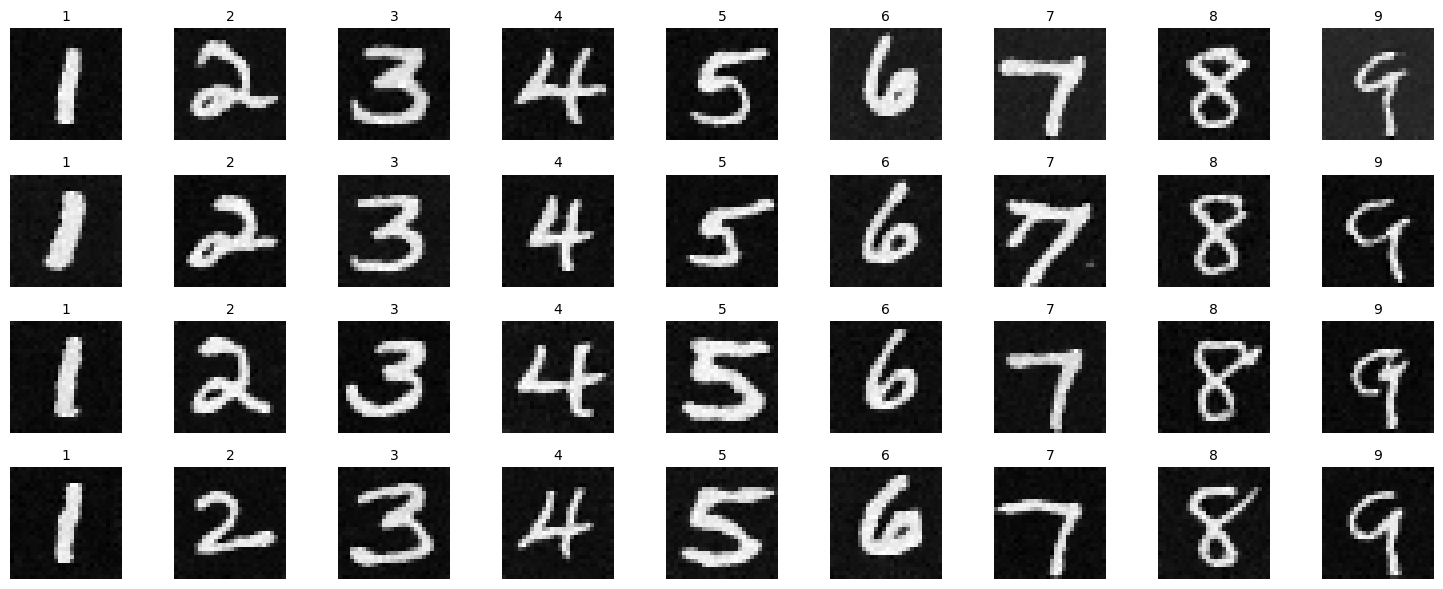
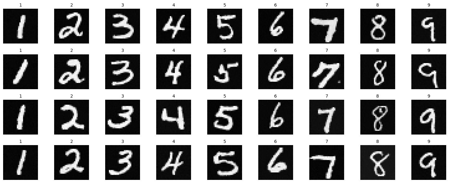
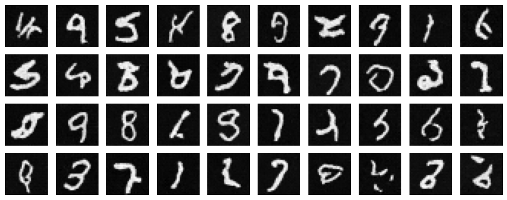
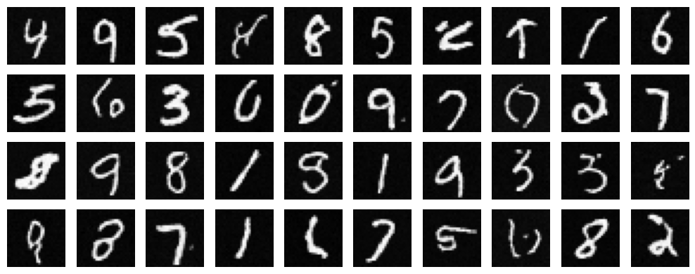
I used a sampling process similar to the DeepFloyd model from part A, except rather than generating the variance I use the beta list. I also generate a blank noisy canvas to produce the sample. Below are samples generated after the 5th and 20th epochs of training. I use the same random seed in order to produce the same numbers, as you can see below the digits from epoch 20 look slightly better than those from epoch 5.
2.4 Adding Class-Conditioning to UNet
For the last model, in order to make the results better and have more control over the generated images, I implemented class conditioning on the UNet for digits 0 through 9. For the conditioning I used a one-hot encoding vector instead of a single scalar. I used the same architecture as part 2.2 except with the addtional condition variable.
2.5 Sampling from the Class-Conditioned UNet
Similar to part 2.3, I generated sampling results for the class-conditioned UNet for 5 and 20 epochs. However, rather than generating random numbers I generate 4 instances of each digit from 0 to 9. Below are the results after 5 and 20 epochs of training. I believe that the samples generated for epoch 20 are better than those generated for epoch 5.
