Part A: IMAGE WARPING and MOSAICING
Introduction
For project 4a, we explored new ways of warping images using homography matrices and generating mosaics between varying frames. The process of generating these images included collecting correspondence points, generating homographies, and compute various warps between an image and its associated homography. The last step was to create a function to generate a mosaic using the warped images. I chose a central image and warped the other images to the defined central image.
Part 1. Shoot the Pictures
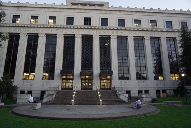
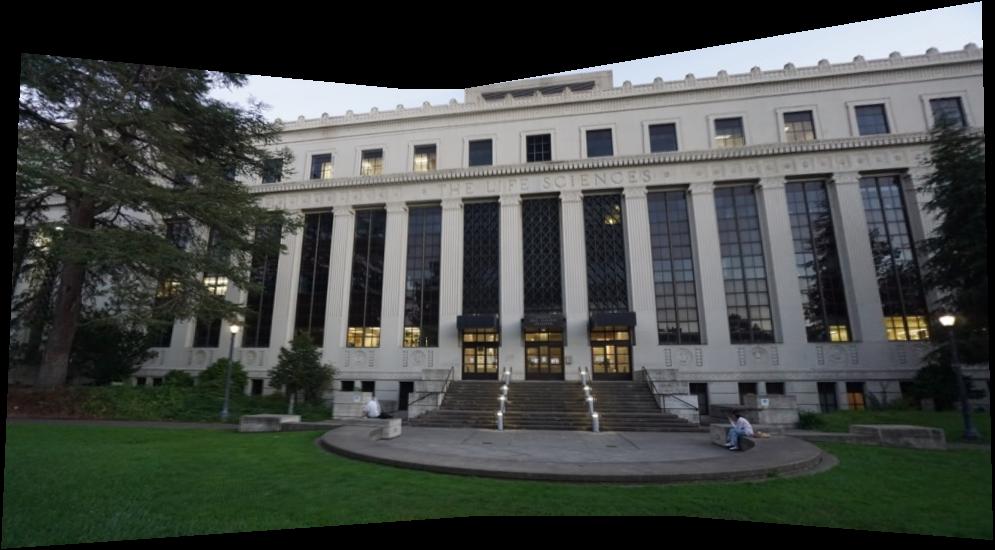
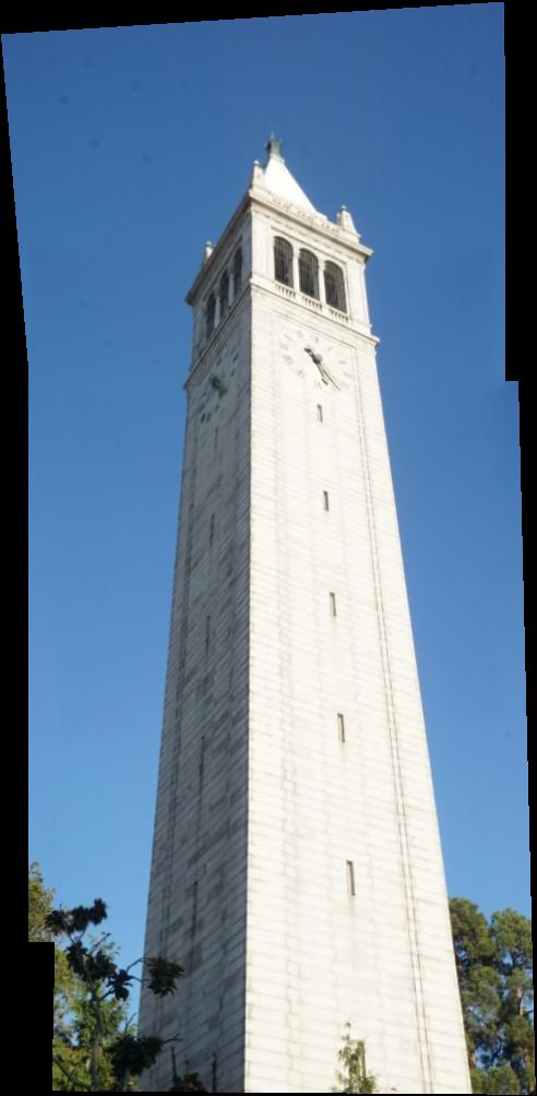
For the first part of this project I took photos from around campus. I tried to fix the center of projection and rotate the camera to capture the pictures of the inside of the Dwinelle courtyard, the campanile, and the outside of valley of life sciences building. I hope you enjoy my generated mosaics.
Images of the Dwinelle Courtyard:
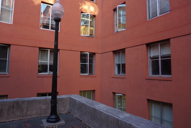
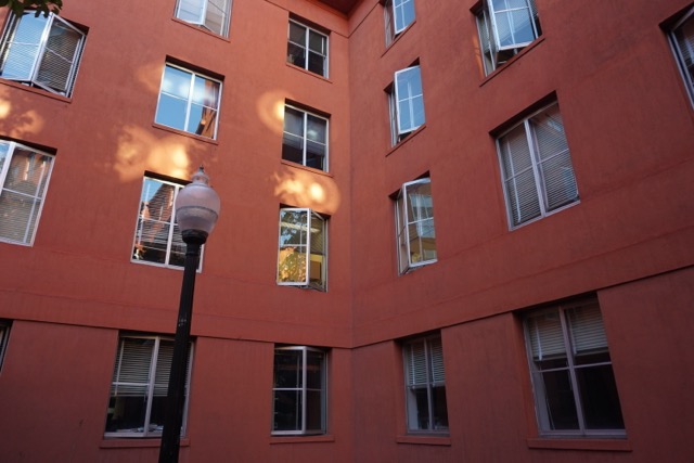
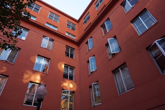
Images of the Campanile:
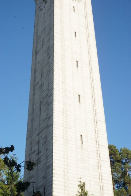
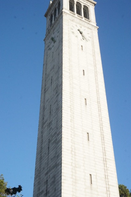
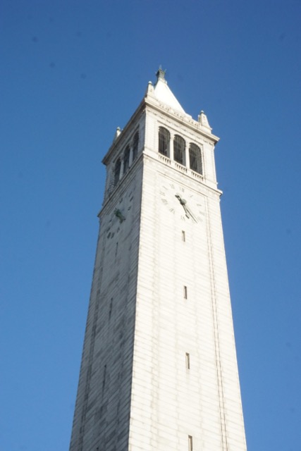
Images of the North side of VLSB:
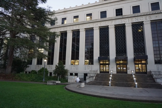
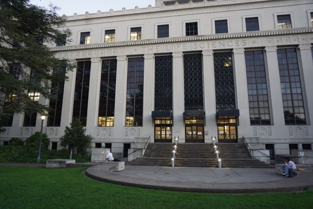
Part 2. Recover Homographies
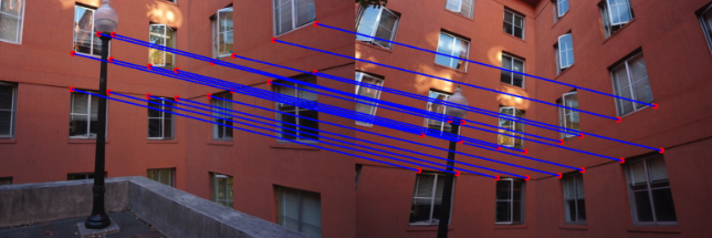
For most of my images I tried to pick correspondence points critical points such as corners of windows or buildings. For my courtyard example, I chose correspondence points based on the corners of windows. I wanted to make a cool visual of the distance between correspondence points of images that are stitched together. I took inspiration from Alec Li's submission from last Fall and using my correspondence plot function from project 3 along with a few changes to generate the following visuals.
Example of correspondence points between two frames
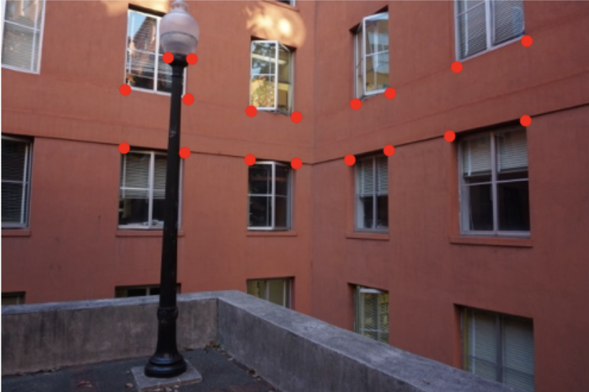
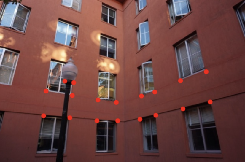
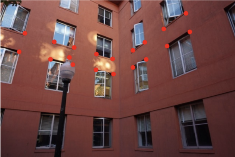
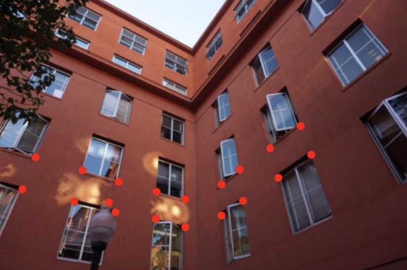

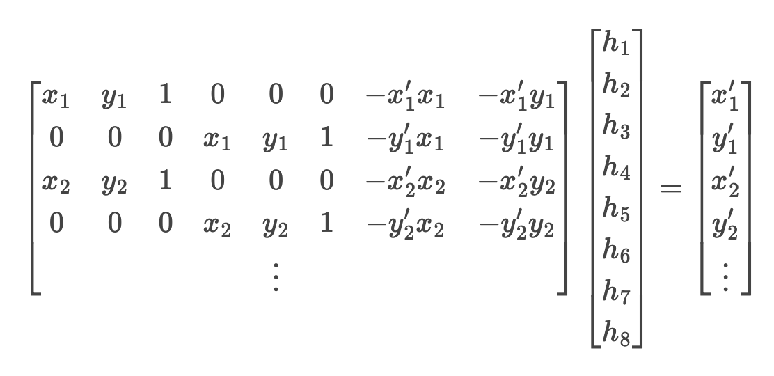
In order to compute the homographies I used the correspondence points I selected for the two input images. I reused the correspondence tool from project 3. I then set up a linear system of n equations based on the n correspondence points. After constructing the system of equations and stacking them in a numpy array. I used numpy's least squares operation to solve for the 8 parameters that solve the system of equations and used these parameters in the homography matrix. I then assign the bottom right to 1 to complete the 3x3 homography matrix.
Part 3. Warp the Images
For my image warp, I used the computed homography to warp an image
towards its corresponding reference image. For my interpolation I
referred to Alec Li's submission from Fall 23 and used the
scipy.interpolate.RegularGridInterpolator function rather than the
scipy.interpolate.griddata.
For the warp, I first generate the grid coordinates for the output
image using np.meshgrid and stacked them using np.stack. Next, I
applied the inverse homography transformation to map coordinates from
the output image back to the input image. Next I generated an input
grid for the interpolation function. The interpolation function I used
requires that the grid be regular. Then I applied the interpolation
function to the x & y input points. I also used extra input parameters
to generate the size of the resulting image. The
RegularGridInterpolator function has a parameter called bounds_error
which I set to false in order to allow coordinates to fall outside the
input image's boundaries but then used the fill_value=0 parameter to
mask these points to account for out-of-bounds coordinates.
Part 4. Image Rectification
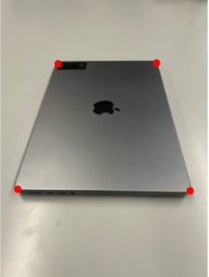
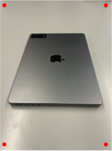
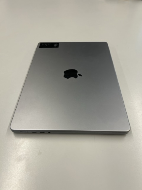
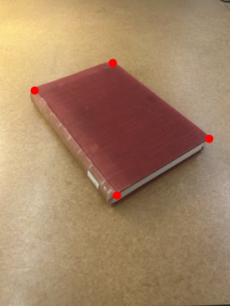
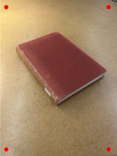
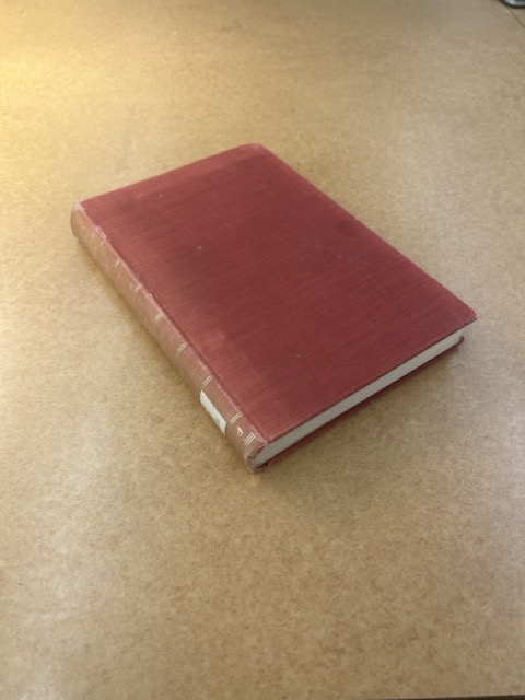
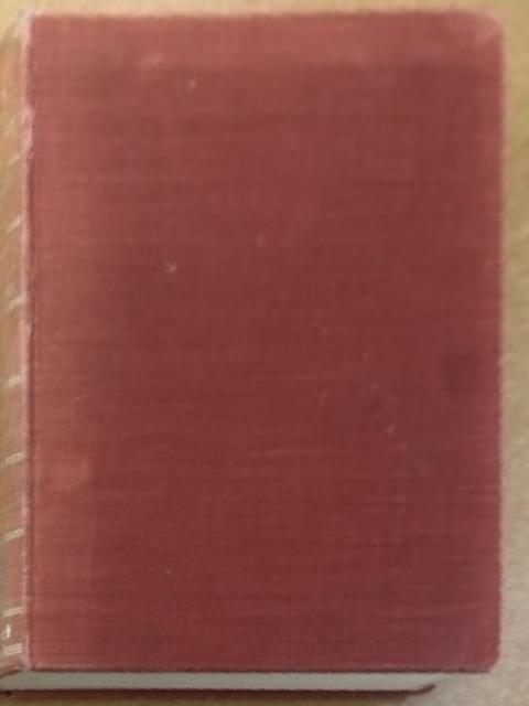
In order to verify my homography and warping function are working I took an angled picture of my computer and of a book in order to rectify them. I chose the correspondence points as the four corners of the original angled object and then used the same image as the second image and chose the correspondence points as a larger rectangle. I then computed the homography of these points and warped the image to produce the rectified images below.

Part 5. Blend the images into a mosaic
For my image mosaic, I used the computed homographies to warp each of
the images in a list to a common projection. I first computed the size
of the final output mosaic by calculating the bounding box using the
transformed corners of each image using their corresponding
homography. My next step was to compute a translation matrix to shift
images into the mosaic frame. I selected one image as the central
image and left it unwarped and warp the other images into its
projection with their homographies. I used a weighted average to
prevent strong edge artifacts.
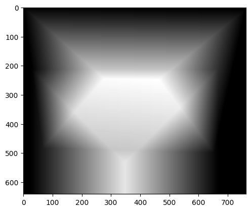
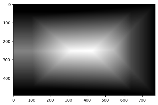
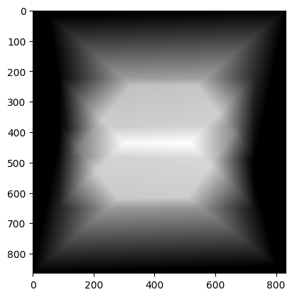
For blending, I created a binary mask for each warped image to
identify which pixels are valid. Next using a hint from ed about
cv2.distanceTransform I computed a blending mask using a distance
transform. This is useful because it is assigns higher weights to
pixels near the image center, and gradually decreases the weight
toward the edges. Once all images are added, I normalize the mosaic by
dividing the accumulated pixel values by the total weights. Lastly, I
divide my mosaic by the weights > 0 to ensure RGB values are between 0
and 1. This completes the smooth blending between the warped images.
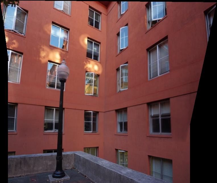
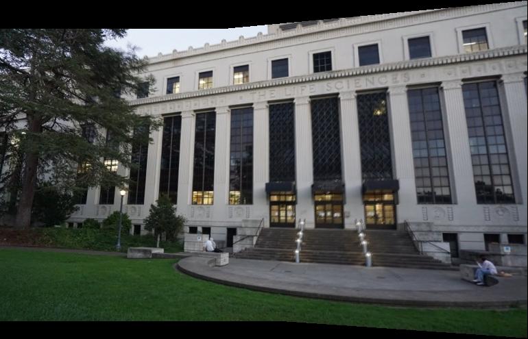
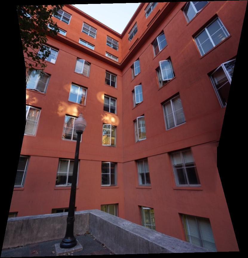
Below I have attached each mosaic and its associated blend mask.
Two image mosaics
I assigned the first image to the identity and the second to a homography from the second to the first.
Example 1


Example 2


Three image mosaics
I assigned the second image as the central image and associated it with the identity matrix as its homography so that it wouldnt be warped. I then computed the homography to project the first image onto the central and project the third image onto the central.
Example 3


Example 4


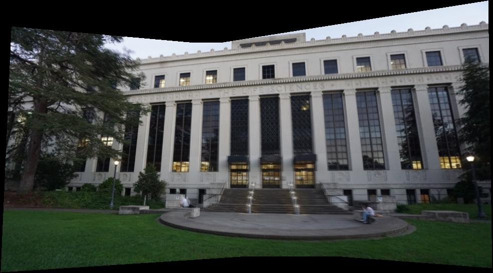
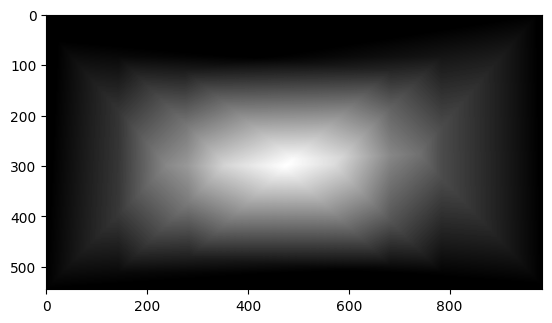
Example 5


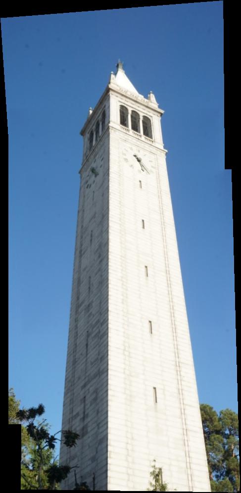
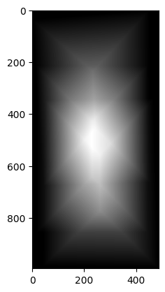
Part B: FEATURE MATCHING for AUTOSTITCHING
Introduction
For project 4b, we create a system for automatically stitching images into a mosaic. We do this by implementing the steps given in the paper "Multi-Image Matching using Multi-Scale Oriented Patches" by, Matthew Brown, Richard Szeliski, and Simon Winder. They explored a new way of image matching unlike previous methods that relied on either direct matching or feature-based, and rather combined these two results in invariant features. The four parts of the paper that are relevant to us include first computing single scale Harris corners to define interest points, although the paper does use multi-scale. Followed by, creating an adaptive non-maximal suppression filter to filter our interest points. Once we have filtered the interest points we can generate feature descriptor for each feature points and match them between two images. Once we compute the points associated with the matched features we can compute a homography using RANSAC. The final step is to compute the mosaic similar to part 4a using the new homography that we have generated.
Detecting Corner Features
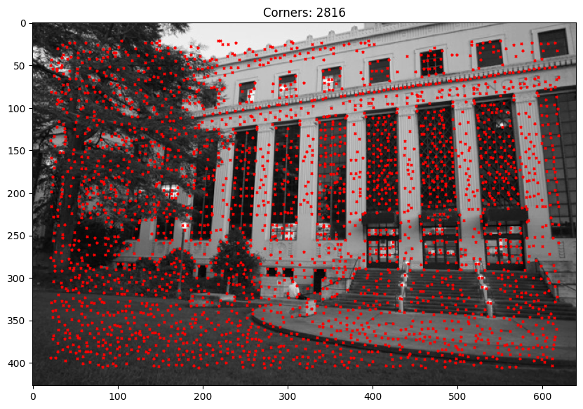
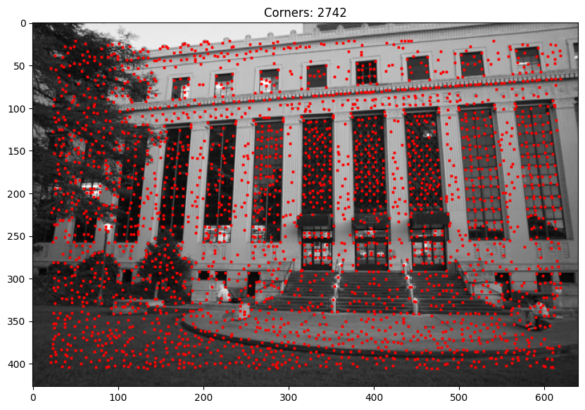
Given that in the instructions we only have to compute Harris Interest points on a single scale, I used the given starter code function from harris.py. Below are two examples of this function in action.
Defining Feature Descriptor
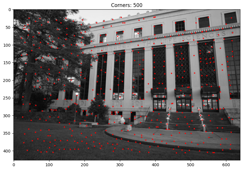
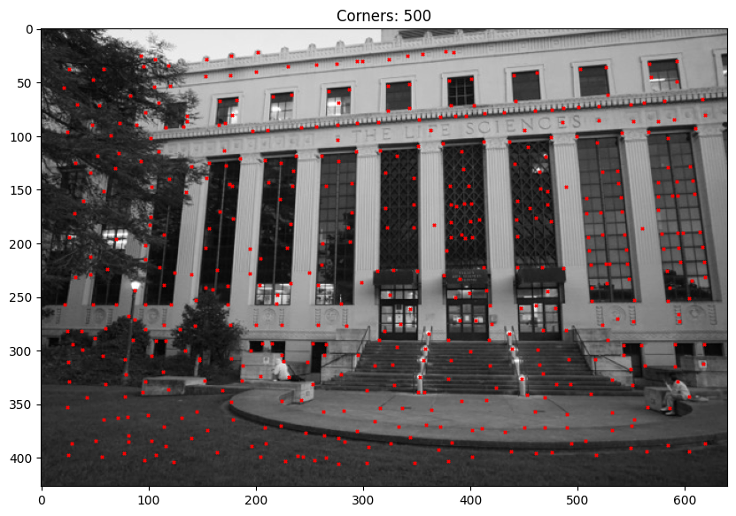
In order to generate the feature descriptors I first created a function to apply adaptive non-maximal suppression or ANMS for short. This function helps to filter the interest points by reducing redundant information while retaining the distribution across the image. Below is an example of the AMNS interest point filtering from the first two example images.
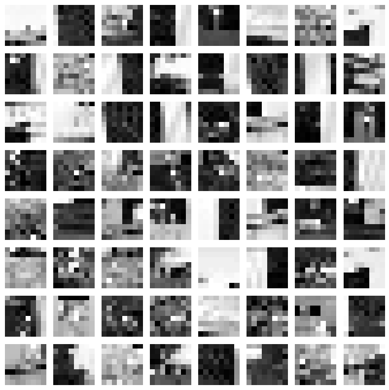
Once I filter my interest points, I then extract the features through sampling patches of size 8x8 from a larger 40x40 window to ensure blurred descriptor's and then I normalize them for the bias/gain. From the paper I also ensure a spacing of s = 5 pixels between sample patches. I selected 64 random patches to display below.
Matching Feature Descriptors
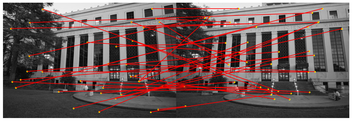
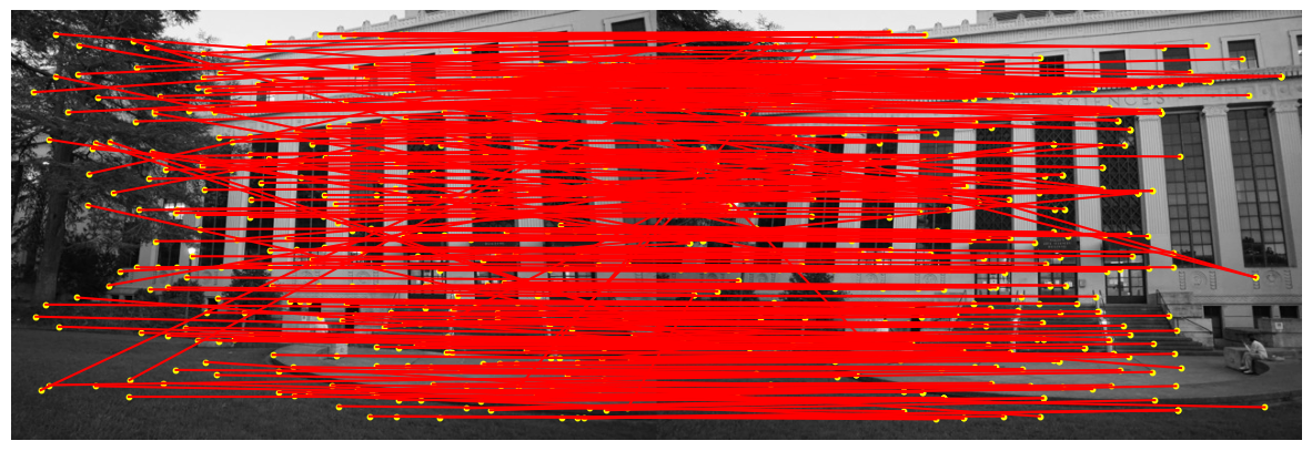
After computing the features for each image, we need to find pairs of features that look similar and are thus likely to be good matches. I matched features between two sets of descriptors using the Lowe's ratio test with various thresholds and found that if the threshold was too low such as 0.2 it would produce a very blurred image. However, if the threshold was set higher to 0.9, it produced a much nicer mosaic with less blur. Below I will attach an image of feature matching on the ANMS points with a threshold of 0.2 and 0.9.
RANSAC Homography
In order to compute the homography I used the 4-point RANSAC algorithm discussed in lecture. In this algorithm I randomly sample 4 pairs of points, and compute the homography for these points. I then store the inliers for each computed homography in a list. After I iterate through the points, I keep the homography that produces the most inliers. The goal is to find the majority transformation.
Mosaic 2.0
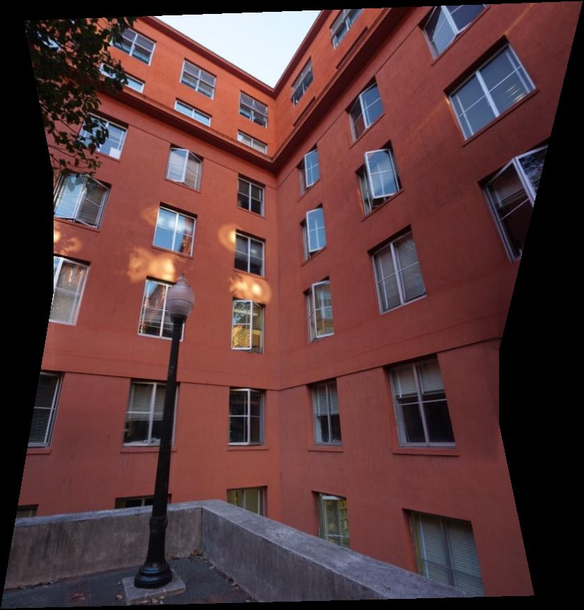
After we compute the homography using the RANSAC algorithm, we can use the same image warp and mosaicing function from part A to produce the final mosaic and compare with the manual correspondence points approach. Below I will attach the 4a results along with the newly computed mosaics.



Reflection
I really enjoyed working on this project and learning how to read and implement a research paper. I think my favorite part was figuring out how to compute the mosaic. From part A, I think the coolest part was computing the rectified images. I hand selected the corners and appropriate output grid and then to validate my warp function applied the warp to the computer and book image with their corresponding homographies. I also enjoyed the linear algebra applications with the homographies and solving the system of linear equations. From part B, I enjoyed reading the research paper, and translating the steps into my code. I think it is a great skill to practice and I plan to try it more it in the future.