Introduction
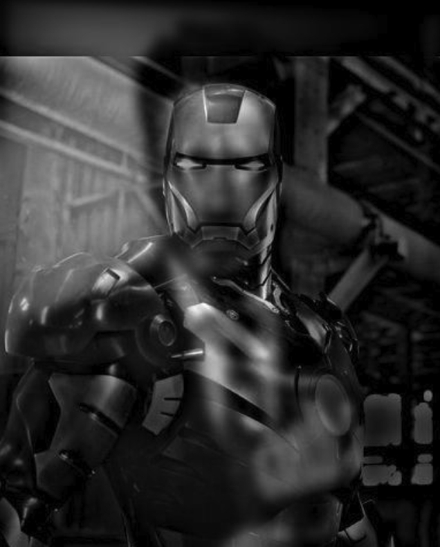
This project explores different ways of using filters and frequencies to alter and combine images. The first portion of the project is examining how images can be sharpened by applying blur, extracting the details, and producing a sharpened image. The next portion was exploring low and high frequency to create hybrid images. The last portion of the project is about Multi-resolution Blending, which means blending together images at various frequencies using Gaussian and Laplacian stacks. Below I am showing a hybrid image that I will explain later on.
Finite Difference Operator
Approach
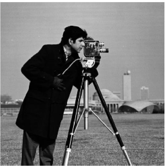
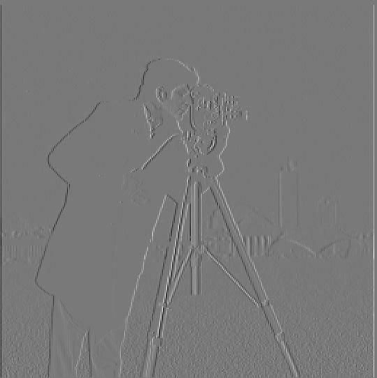
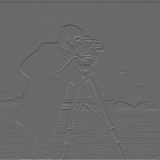
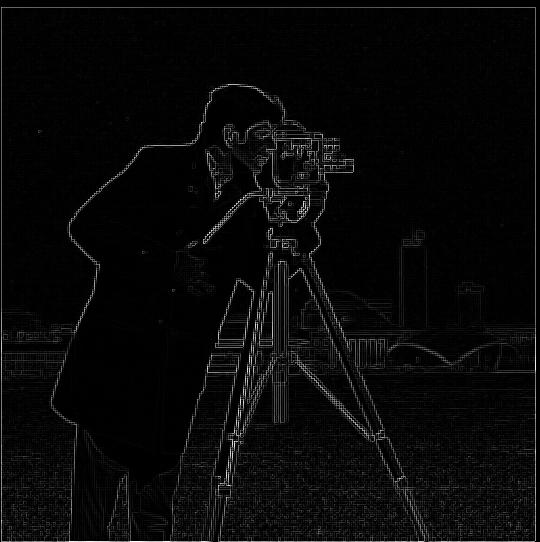
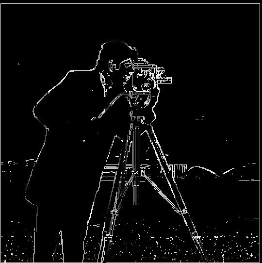
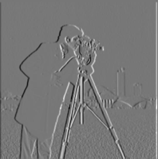
In the first part of this project I generated finite difference operators D_x and D_y, where D_x = np.array([[1, -1]]) and D_y = np.array([[1], [-1]]). I then used the two kernels to convolve an image using scipy.signal.convolve2d to produce images of their respective partial derivatives partial_x and partial_y which would generate the edge image. Then I calculated the gradient magnitude image using np.sqrt(partial_x ** 2 + partial_y ** 2), treating the pixel values of the partial derivative images as elements of the gradient vector and taking its L2 norm as the final pixel value.
Gradient magnitude
The gradient magnitude computation is np.sqrt(partial_x ** 2 + partial_y ** 2), where partial_x and partial_y are the partial derivatives in the x and y directions. We compute the gradient magnitude of the image in order to generate an edge image. Using a threshold in order to classify what should be considered as an edge.
Derivative of Gaussian (DoG) Filter
1.2.1 Blurred Finite Difference

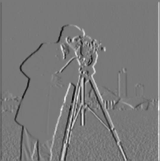
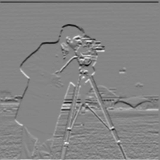
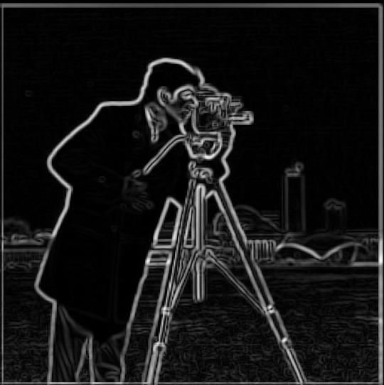
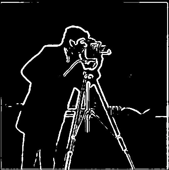
What differences do you see?
Between the original and blurred image, it seems that the blurred image amplifies the edges because of the thicker lines. Where as the original image has more detailed edges, as well as more noise. I also noticed that for the blurred image results the lines are more smooth where as for the original image the lines are more sharp.


1.2.2 Derivative of Gaussian

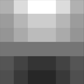
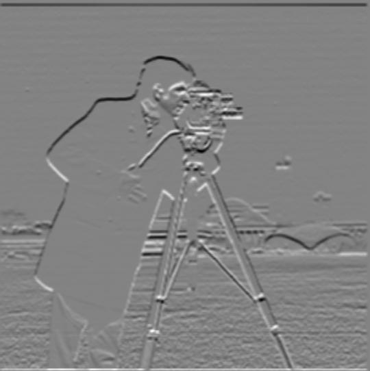
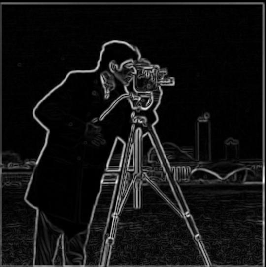
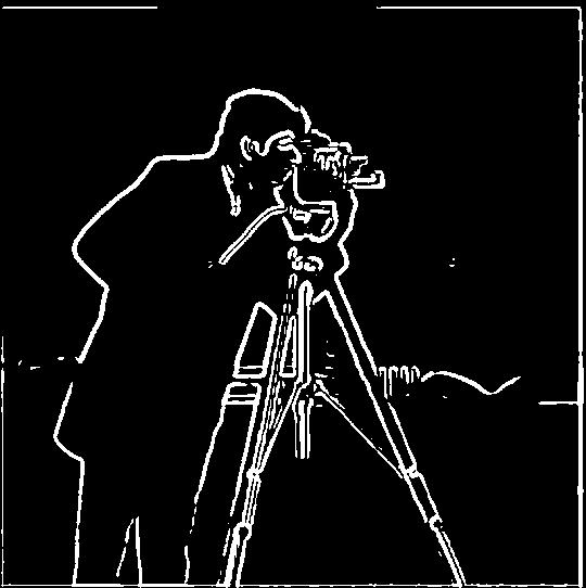
Comparison
It seems that the results are identical between the binarized blurred finite difference gradient magnitude and the binarized derivative of Gaussian gradient magnitude. There are a few points of noise that are different between the two images.


Image Sharpening
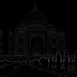
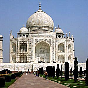
The next portion of this project involved sharpening images. This can be done by passing a input image through a low pass Gaussian filter to generate a blurred version. In the low pass filter, I parse the image into it's three channels, applying the gaussian to each channel, and then merge the image back together. Next in order to generate the detail of the image, we subtract the blurred version from the original image. Then in order to create the final sharpened image I used the following formula: sharpened = image + alpha * detail. The alpha I used was 1.5 for the taj image.
Process
Below I show an example of the sharpen workflow, I first blur the image, then extract the detail, and then sharpen the original image.
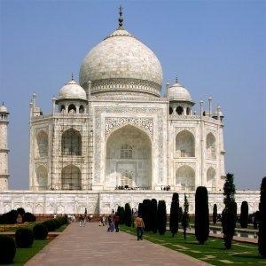

Results

Hybrid Images
For the second part of this project we had to create hybrid images, which takes in a two images, one that will go through a low pass filter and one that will go through a high pass filter. The low pass is applied in the form of a gaussian blur using the recommended getGaussianKernel() with the kernel size equal to 6 * sigma. The high pass filter is created by first running the second image through the low pass filter and then passing the blurred image with the original into the high pass in order to perform the following calculation: detail = original - blurred. The last step is to average together the two images to produce the hybrid image.
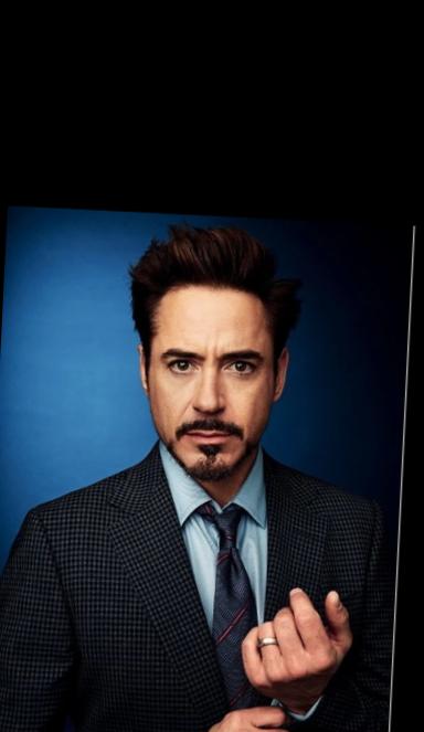
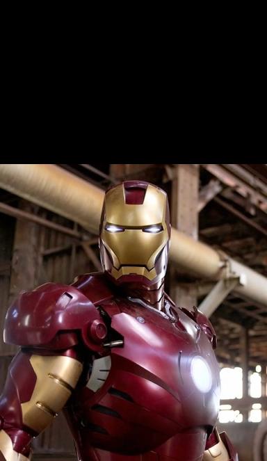
I thought it would be cool to create a hybrid image of Robert Downey Jr. and Ironman, because he is one of my favorite super heros. For this hybrid image I used a low sigma of 5 and a high sigma of 5 too.
Process
Below I first show the two aligned images, then the low pass of the first and the high pass of the second, followed by the genrated hybrid image.
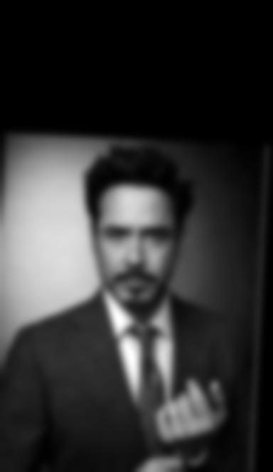
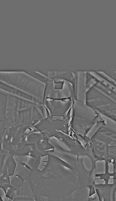
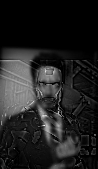
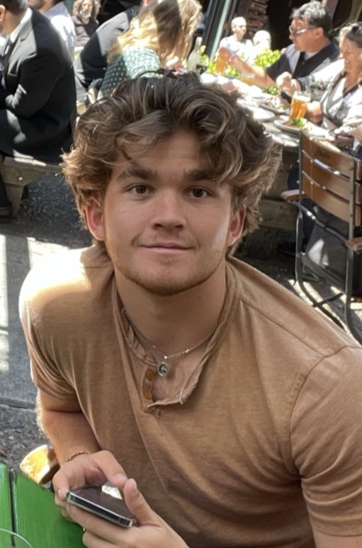
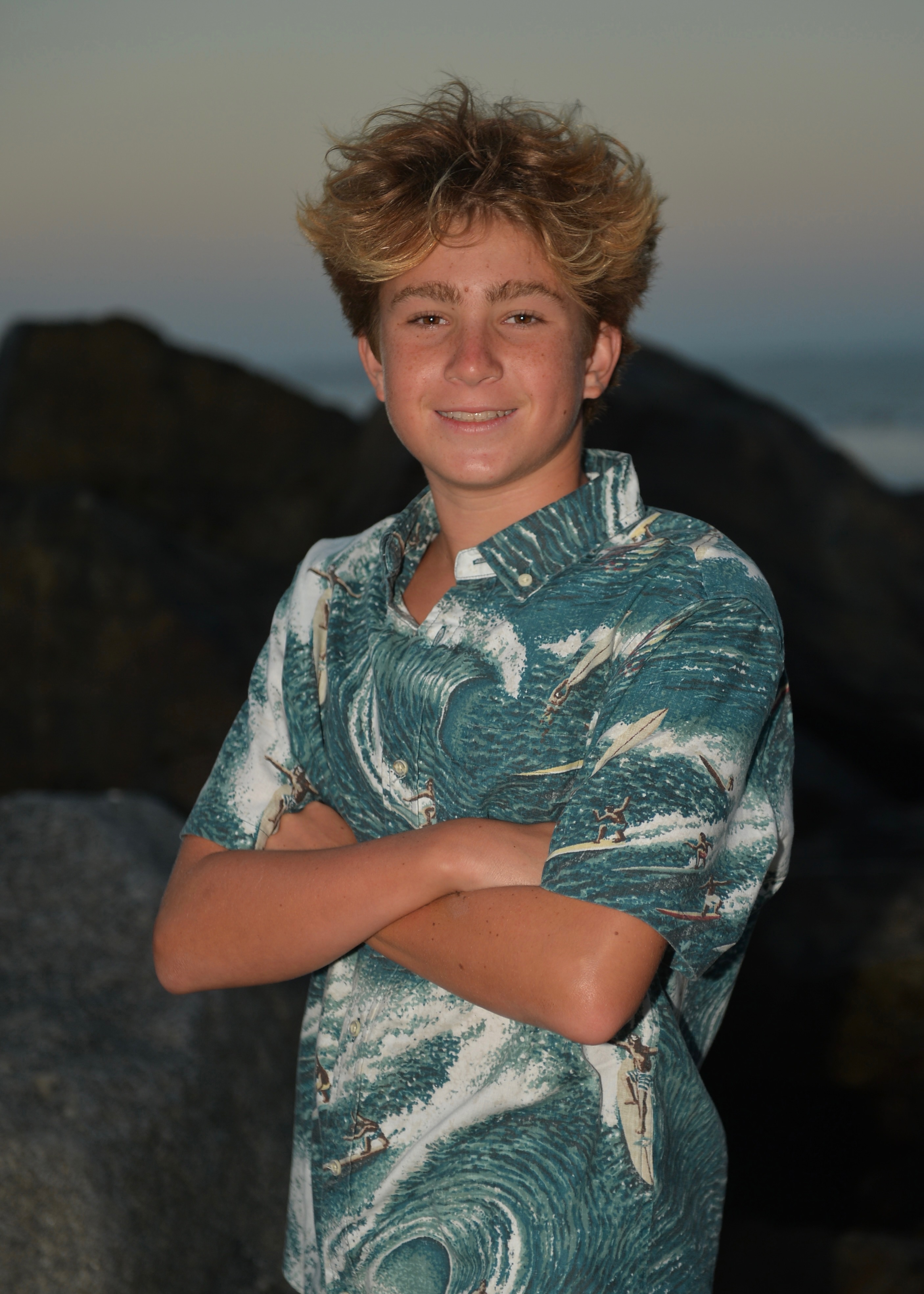
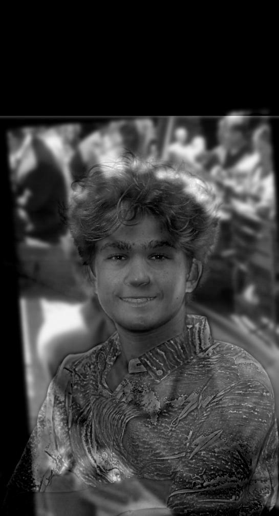
For the past 10 years my family and friends have always said that my brother looks like a younger version of myself. So I thought it would be fun to create a hybrid image of him now (he's a freshman in high school) and a picture of myself from a few years ago. For this hybrid image I used a low sigma of 4 and a high sigma of 4 too.
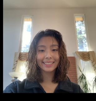
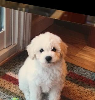
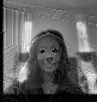
Unfortunately when I tried to created a hybrid image between Jossie and her puppy, I dont think it worked well. This may be due to the dark coloring of the puppies nose, and therefore I consider this one a failure. For this hybrid image I used a low sigma of 2 and a high sigma of 4 too.
Fourier Transform
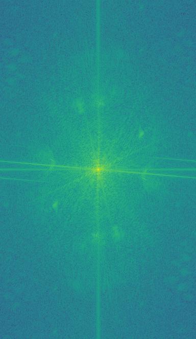
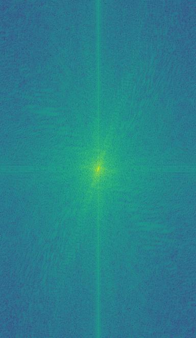
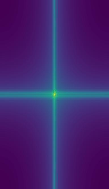
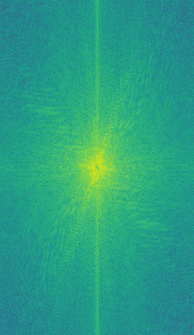
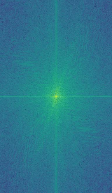
For the Ironman hybrid image, another cool analysis is with the Fourier transform. I applied it to the original images, then both the low and high frequency image and finally to the hybrid image. This produced the following images:
Gaussian and Laplacian Stacks
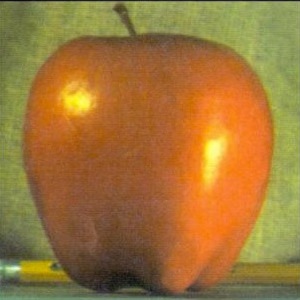
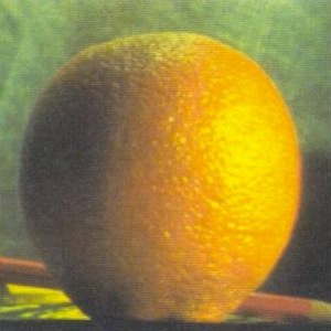
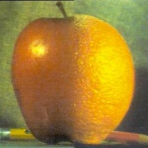
For this portion of the project, rather than creating a gaussian or laplacian pyramid, I generated a stack. This means that we do not have to scale down our image in between each layer. The gaussian stack progressively blurs the inputted image with Gaussian filters and a increasing sigma value. The laplacian stack computes the difference between each adjacent level in the Gaussian stack. The difference represents the high-frequency details lost between each level of blurring. The final level of the Laplacian stack is the same as the last level of the Gaussian stack. In order to visualize the intermediary steps of the laplacian, I had to normalize the output of the laplacian stack with a min max normalization. Below I have attached the gaussian and laplacian stacks. I define a level and sigma variable to alter the results of the stack functions.


The creation of the ORAPLE! I set levels to 5 and sigma to 2 to generate this blended image.



Multiresolution Blending
We first input two images (im1 and im2) and a mask image, and compute the gaussian stack and laplacian stack for both of these images. Next we create the gaussian stack for the mask. Once the stacks are generated we can blend the images at each level across the three stacks. The formula would be, blended = (1 - mask_g_stack[i]) * im1_l_stack[i] + mask_g_stack[i] * im2_l_stack[i]. Then once we have created the blended stack we have to reconstruct the blended image by combining the layers of the blended stack.
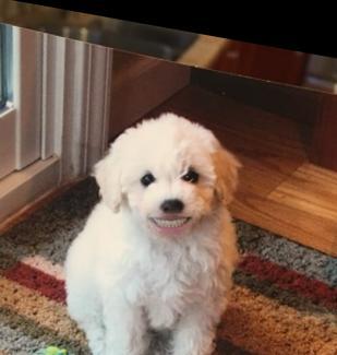
For my first blended image, I thought it would be fun to put Jossie's smile on her puppy. Since the hybrid image did not work earlier, I thought I would create a mask to cut out her smile and cropped into onto Muppynyo's image.



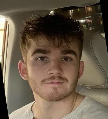
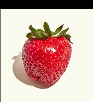
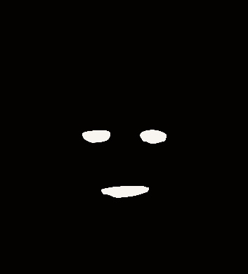
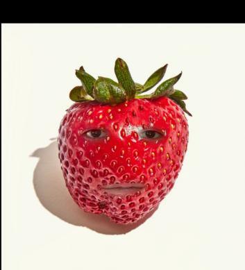
For my second blended image, I saw that on a submission from fall 23 a student put their face on an apple, so I thought it would be fun to do something similar with a strawberry. I created a mask with a cutout of my eyes and mouth and the applied the same blending function to the two images and mask.
