Project 1: Poor Man's Augmented Reality

Introduction

For my first final project I chose the augmented reality project and used a rubiks cube as my platform since it had a natural grid that I could plot the correspondence points. After plotting the 2D points on the rubiks cube, I manually labeled the 3D points of the cube. This allowed me to compute a projection matrix and a 3D space axis as I will show below. After computing the 3D space of the cube, I project a 3D cube onto the top of the rubiks cube.

Input Video

I initially attempted to draw a rectangular grid on a shoe box but then struggled to get the distance of the points to match on height and width. So I decided to pivot and use a rubiks cube since it had a natural grid. Below is a video I took going around the rubiks cube.

Keypoint Selection

Next I extracted the first frame of the video and computed the keypoints located at all of the critical sections on the cube. I intentionally removed a few of the points as they began to move as the side of the cube goes out of frame in the following part. I computed 29 critical points and computed that the length of the cube was 2.1 inches and the distance between each points was 0.7.

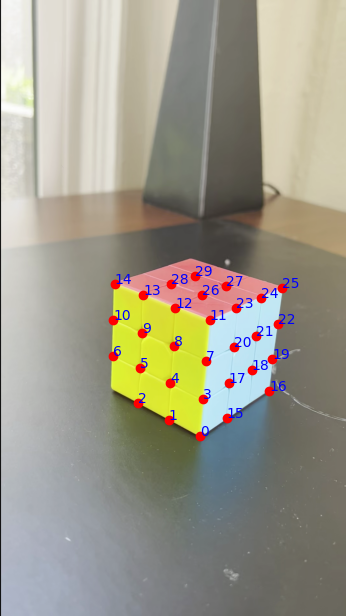
Keypoints with known 3D world coordinates

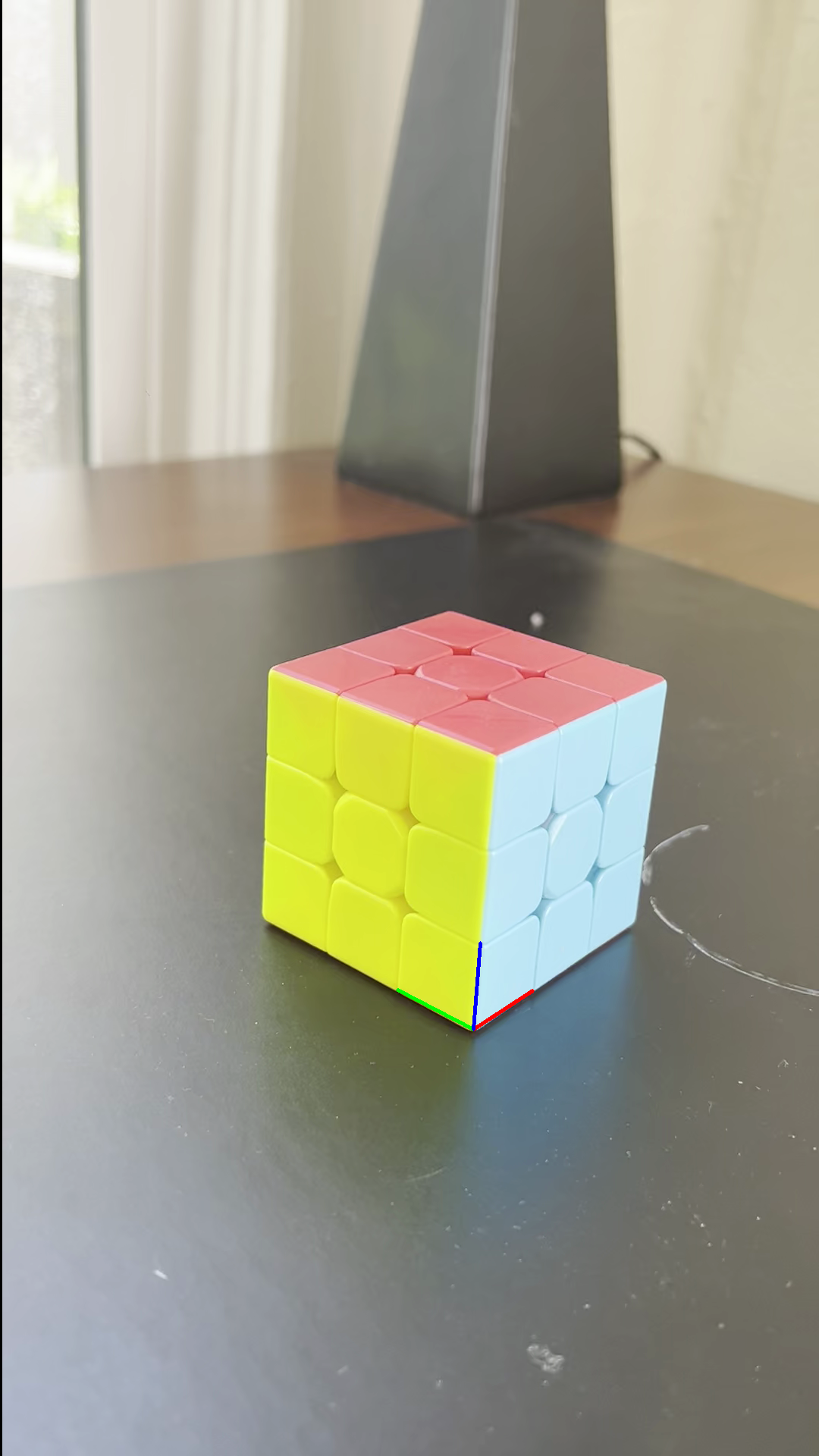
Next I compute the camera projection matrix and deine the corrected 3D axis points. I then draw the 3d axes on the frame given that (0,0,0) starts at the bottom corner which I intentionally made as the first point in the array.

Propogating Keypoints to other Images in the Video

After calculating the projection matrix and computing the axes, I used an off the shelf tracker, cv2.calcOpticalFlowPyrLK() to propogate keypoints to the other frames of the video. This off the shelf tracker uses the Lucas-Kanade method to track the keypoints. I use the optical flow estimation to maintain the correspondence between the 3D points and their 2D image projections per frame. Once the keypoints are tracked for each frame, I apply solvePnP() to estimate the camera pose for that particular frame.

Projecting cube in the Scene

Once I solved for the camera projection matrix which maps the 2D image coordinates to their 3D coordinates of points in the world. I then decompose the projection matrix into the intrinsic camera parameters using cv2.decomposeProjectionMatrix(). These intrinsic parameters include the camera's focal length, principal point, and orientation in space.

After I computed the projection matrix and computed the camera intrinsic parameters, I project a 3D cube onto four of the points on the top of the rubiks cube. To do this, I first define the cube in local coordinates and then map it into the world coordinate system by using the direction vectors derived from the selected four points. With the camera intrinsics fixed, I track the reference points frame-by-frame using the optical flow function as mentioned above. I then apply solvePnP() to update the camera's pose for that frame, and then projectPoints() to place the 3D cube consistently in the scene. This allows me to compute a 3d artificial cube on top of the rubiks cube.

Project 2: High Dynamic Range

Introduction

For my second project I worked on the High Dynamic Range imaging project from Brown University. This project included starter code as well as various sets of stationary images. I used the starter images to create a radiance map and then tone map the images to produce the HDR images. I then used the Durand tone mapping function to produce the final results which I have attached below.

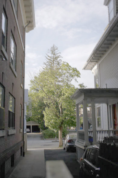
Input Images

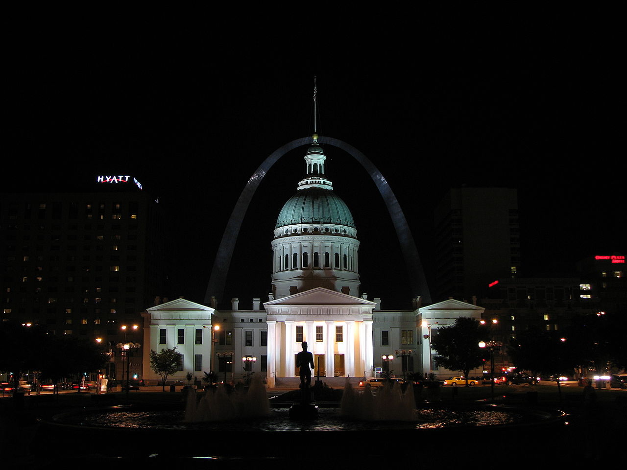
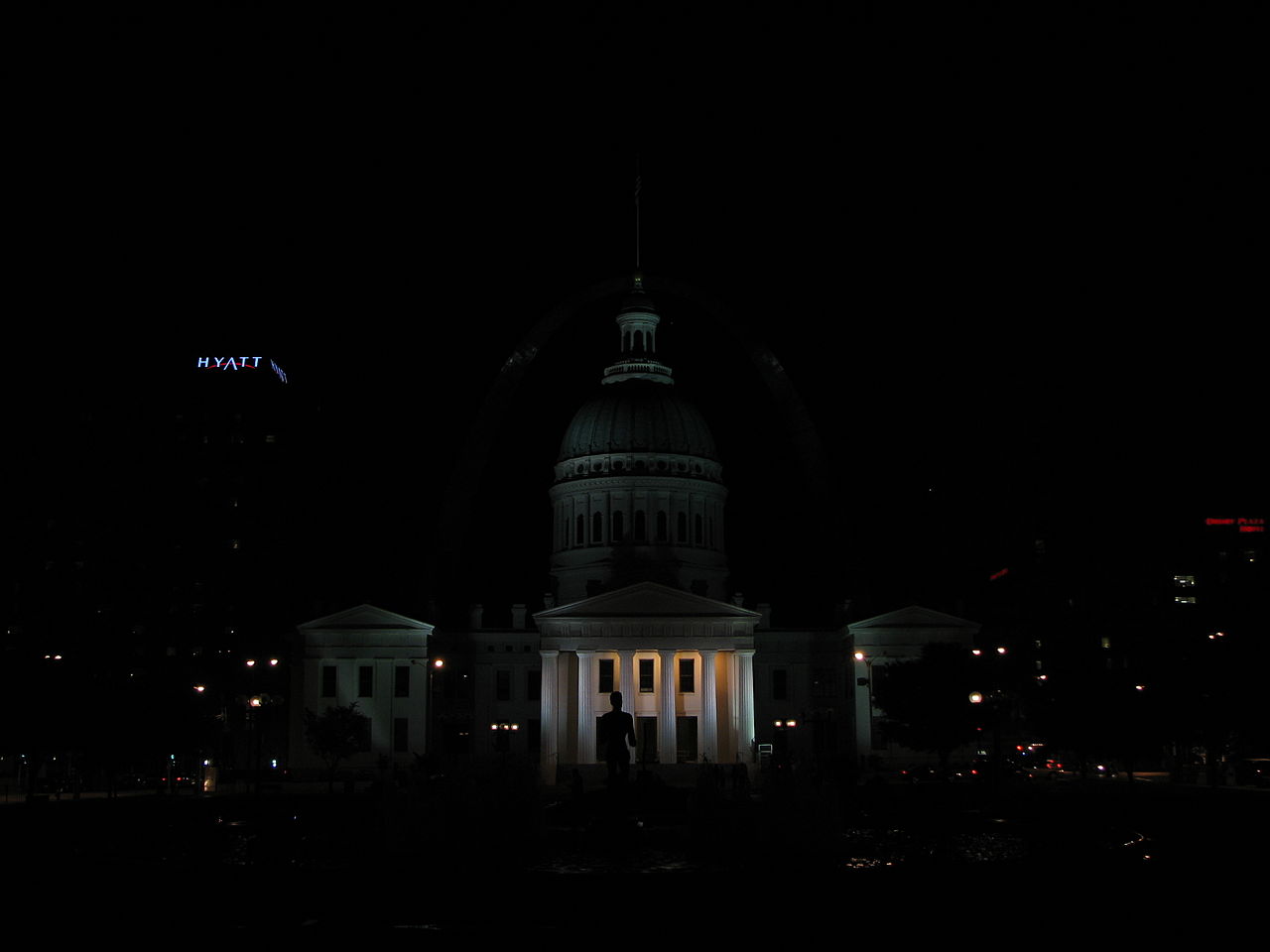
The starter images are all various scenes with multiple captures at varying exposures. The longer the exposure, the more light is captured.

Radiance Map Construction

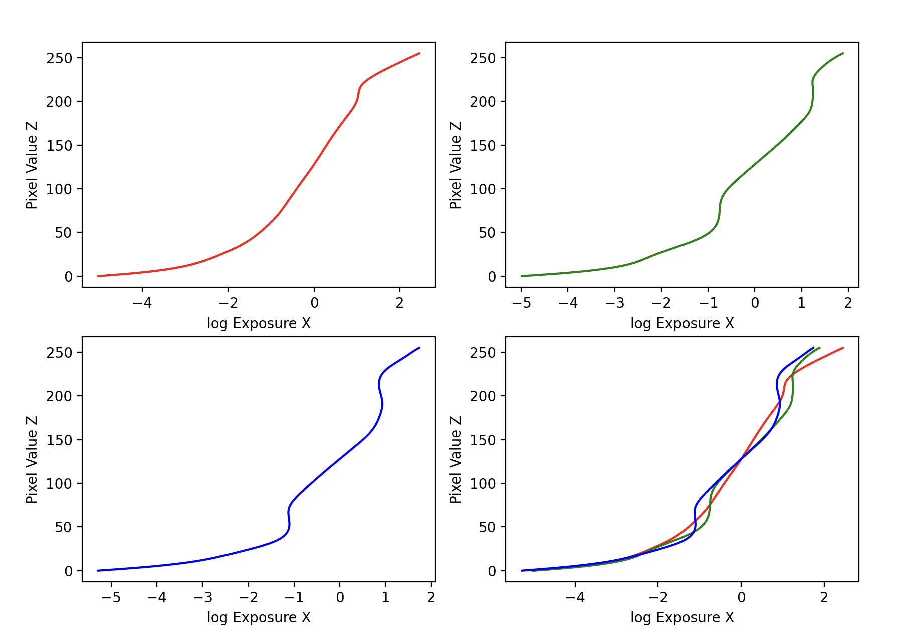
The observed pixel value Z_ij for pixel i in image j is a function of unknown scene radiance and known exposure duration: Z_ij = f(E_i Δt_j). Here, E_i is the unknown scene radiance at pixel i, and scene radiance integrated over some time E_i Δt_j is the exposure at a given pixel. In general, f might be a somewhat complicated pixel response curve.

By implementing the solve_g() function which returns the imaging system's response function g as well as the log film irradiance values for the observed pixels. This maps from pixel values (from 0 to 255) to the log of exposure values: g(Z_ij) = ln(E_i) + ln(t_j) (equation 2 in Debevec). Given that the images are stationary across all frames the scene radiance E_i is constant for a given pixel across all images, and the exposure time t_j is known.

Next I implemented the hdr() function which takes in the imaging system's response function g (per channel), a weighting function for pixel intensity values, and an exposure matrix containing the log shutter speed for each image, and reconstructs the HDR radiance map using the description in section 2.2 of Debevec. This includes the following formula: ln(E_i) = g(Z_ij) - ln(Δt_j). (equation 5 in Debevec)

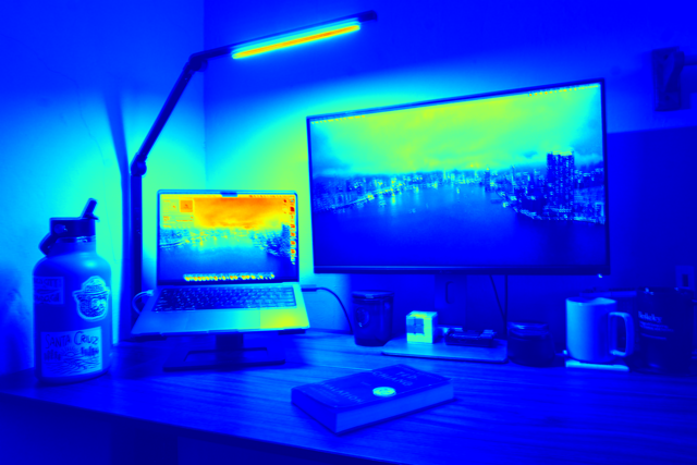
Tone Mapping

After I computed the HDR radiance map, the next step was to implement tone mapping which compresses the dynamic range of an image allowing you to see detail in both bright and dark regions. I implemented two mapping operators, the first one is called Global simple which applies a pixel-wise transform: E_i' = E_i / (1 + E_i) and then I also normalized the results. The second one is called the Durand operator which I implemented using the following steps. First I compute the intensity which is the mean of hdr_radiance_map. Next I compute chrominance channels which seperates the channels into R,G,B and computes each channel divided by the intensity. Next I compute the log intensity to use in the cv2 function bilateralFilter() then we can compute the base layer. After that I scale the base layer and reconstruct the log intensity and then convert back to linear scale. I then reconstruct the color channels and stack them. Finally I normalize the results, and apply a gamma correction.

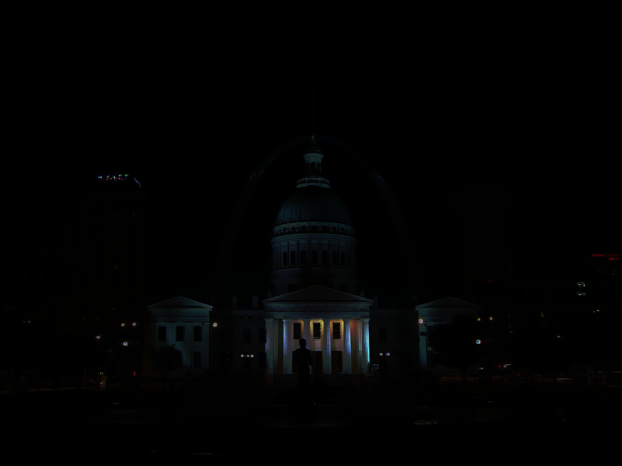
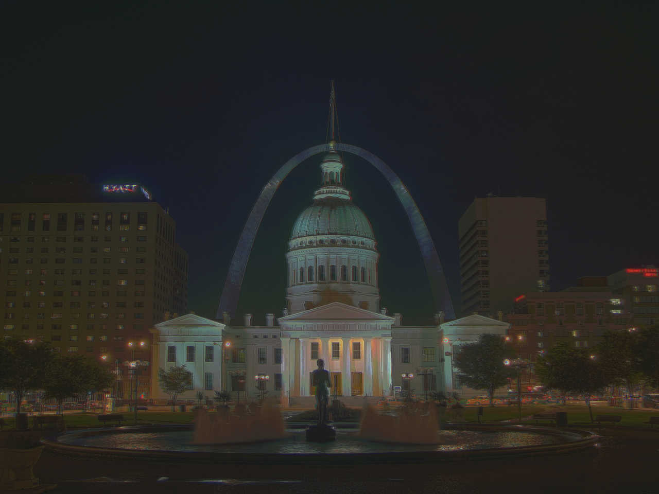
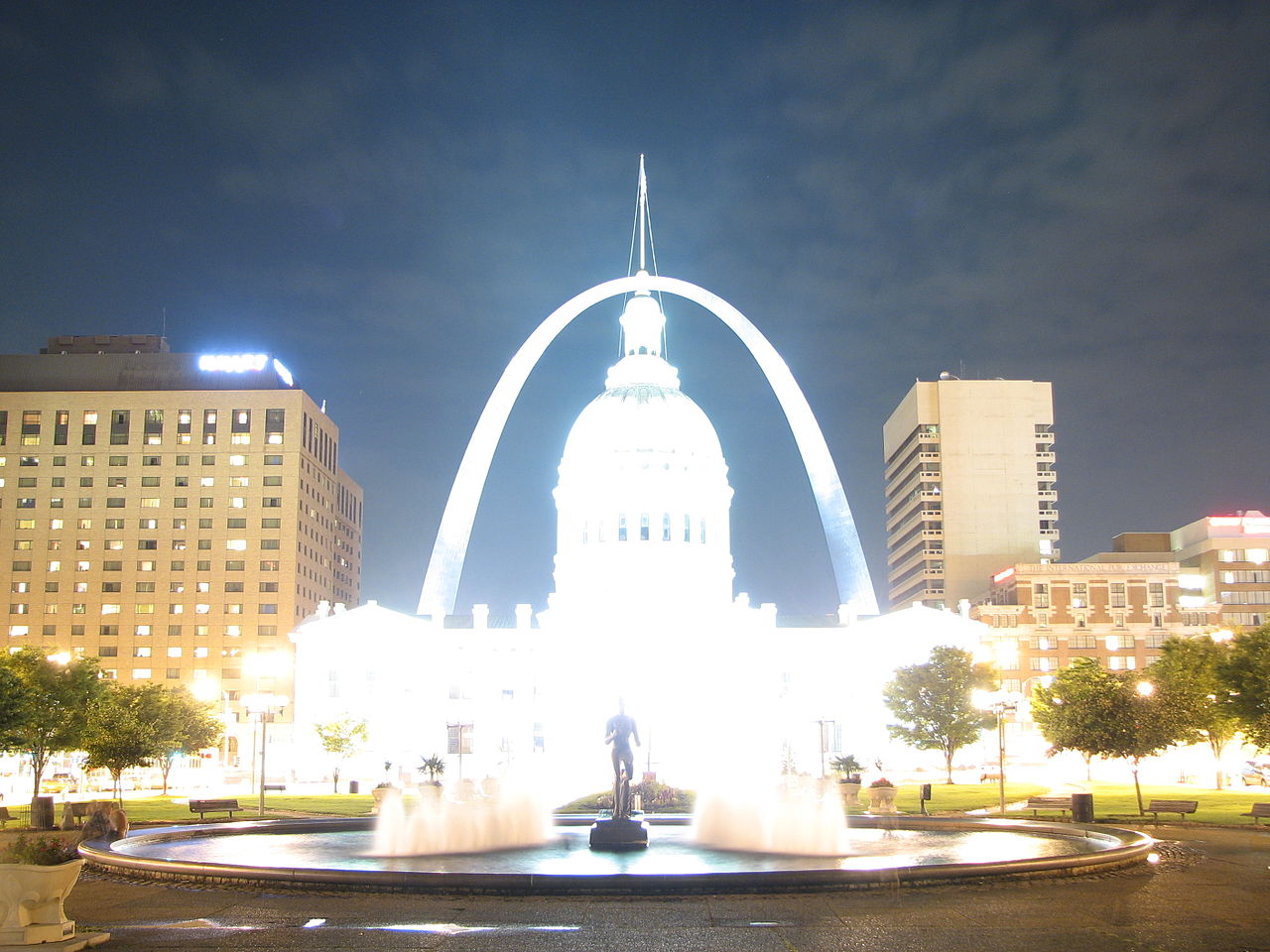
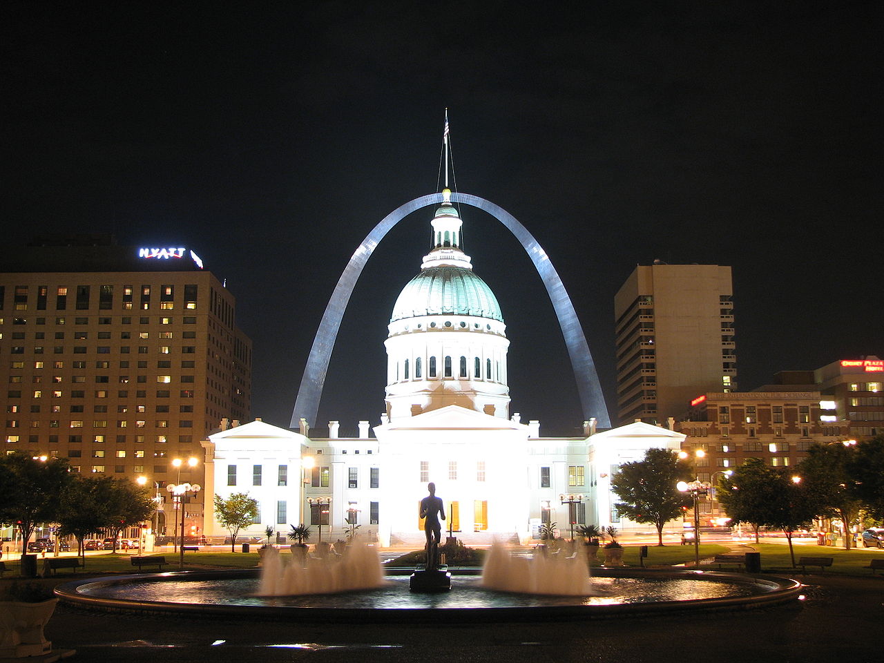
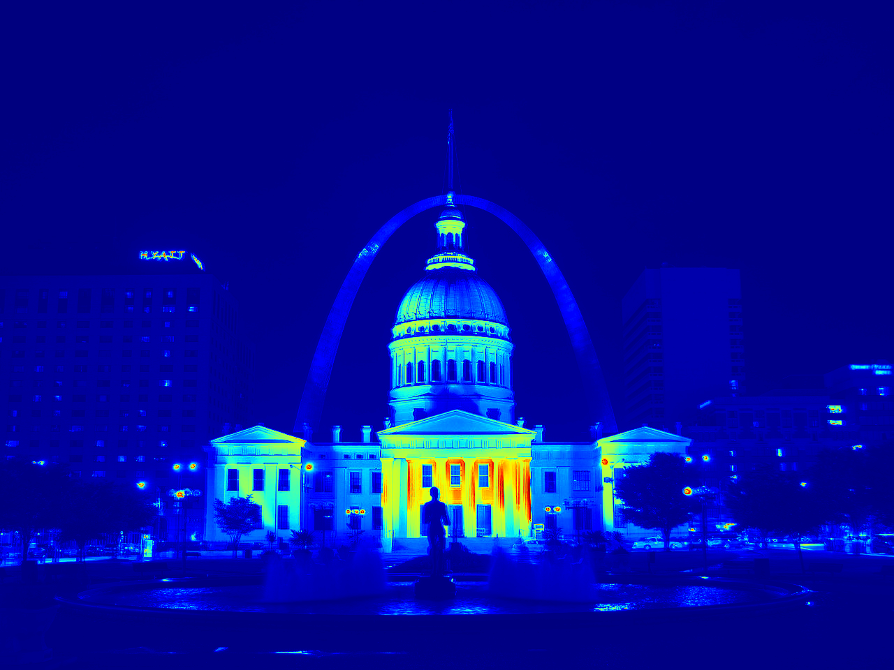
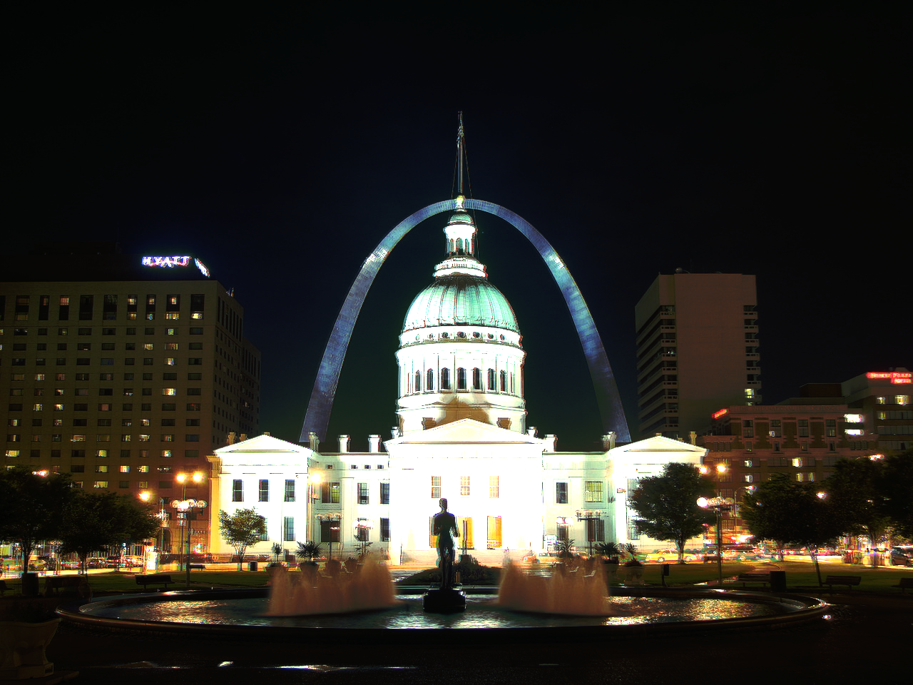
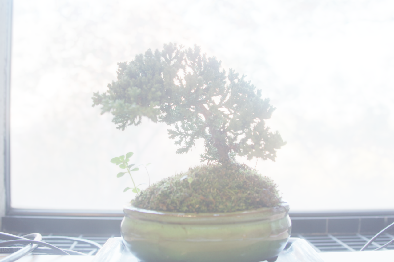
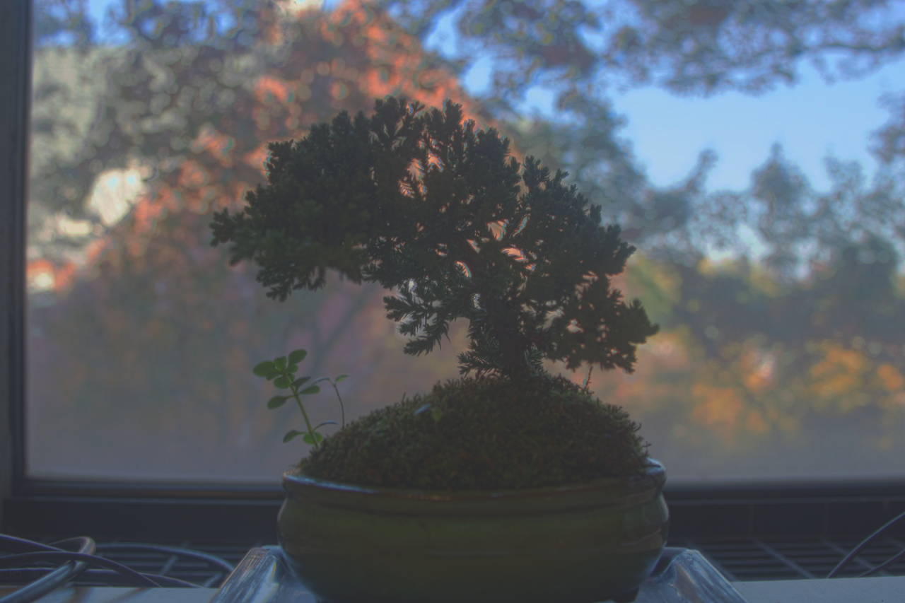
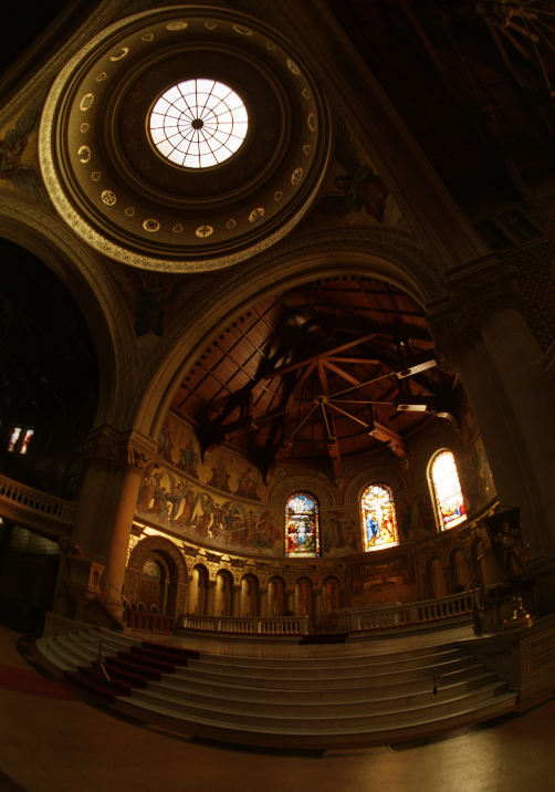
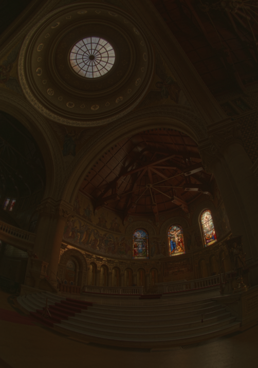
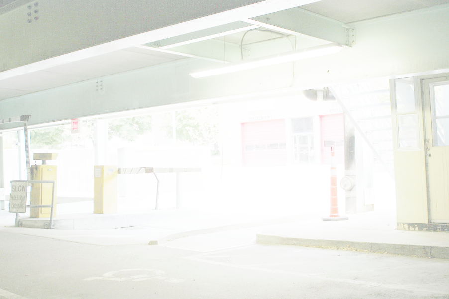
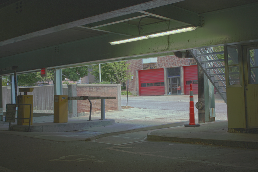
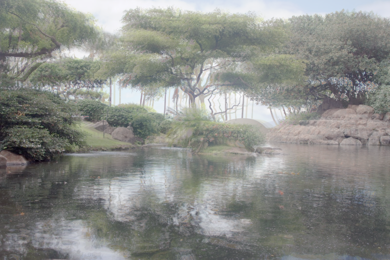
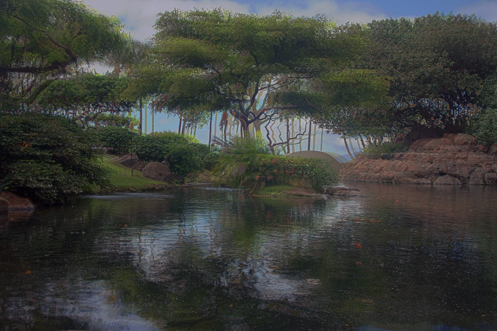
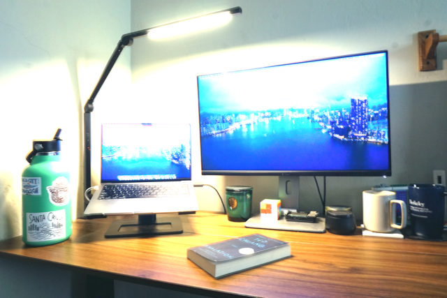
HDR Results

Below are my results which include the global simple and durand output for the Arch, Bonsai, Chapel, Garage, Garden, House, Mug, and Window photo sets. For Garden and House photos, I normalized in the HDR function while in log space in order to produce a better simple and Durand image. I used a gamma variable of 0.5 in my Durand function in the cases where I needed to normalize in the log space. Where as, for the other images I used a gamma of 2.5 in the Durand function in order to increase the brighness of the image.

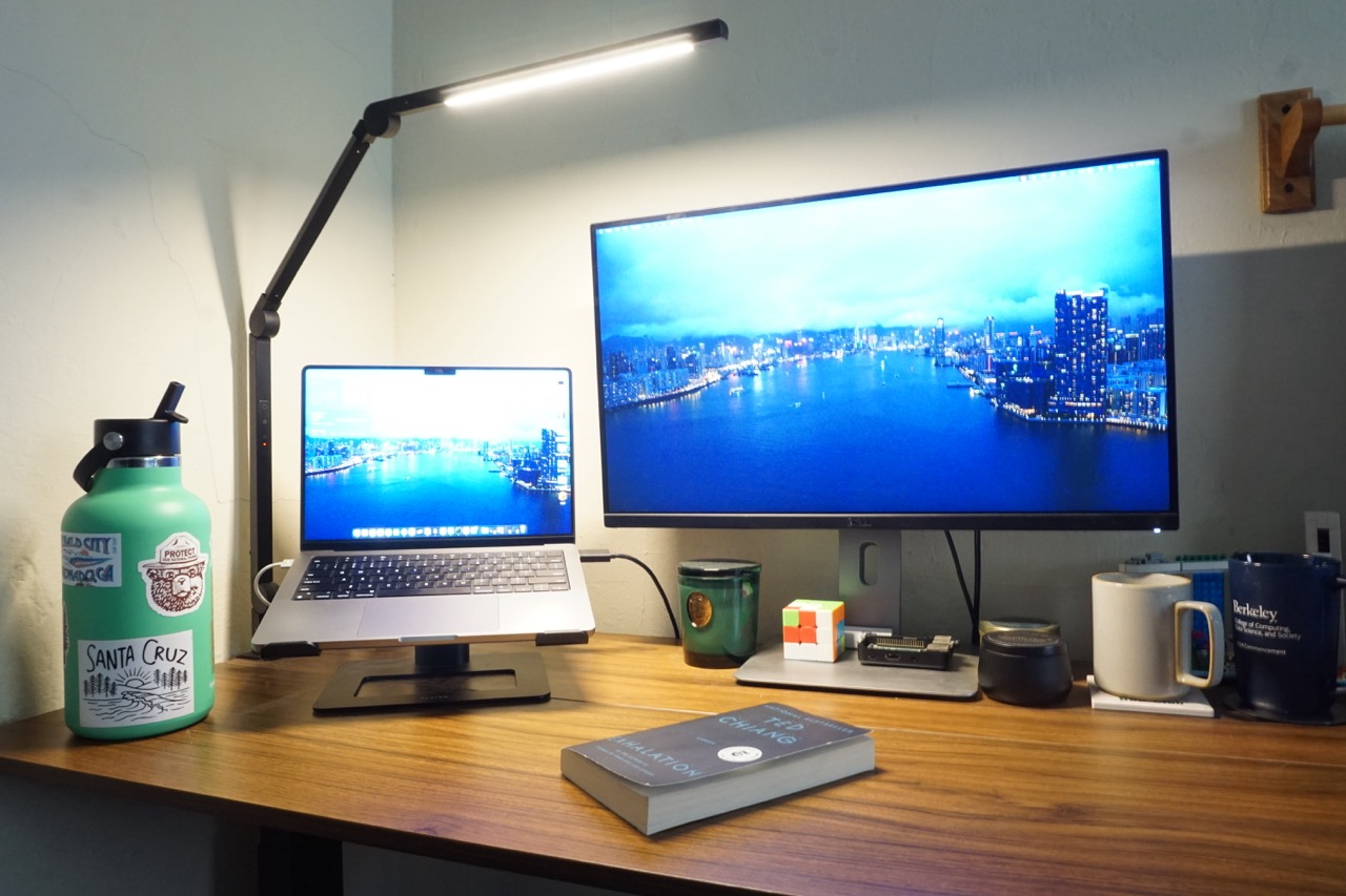
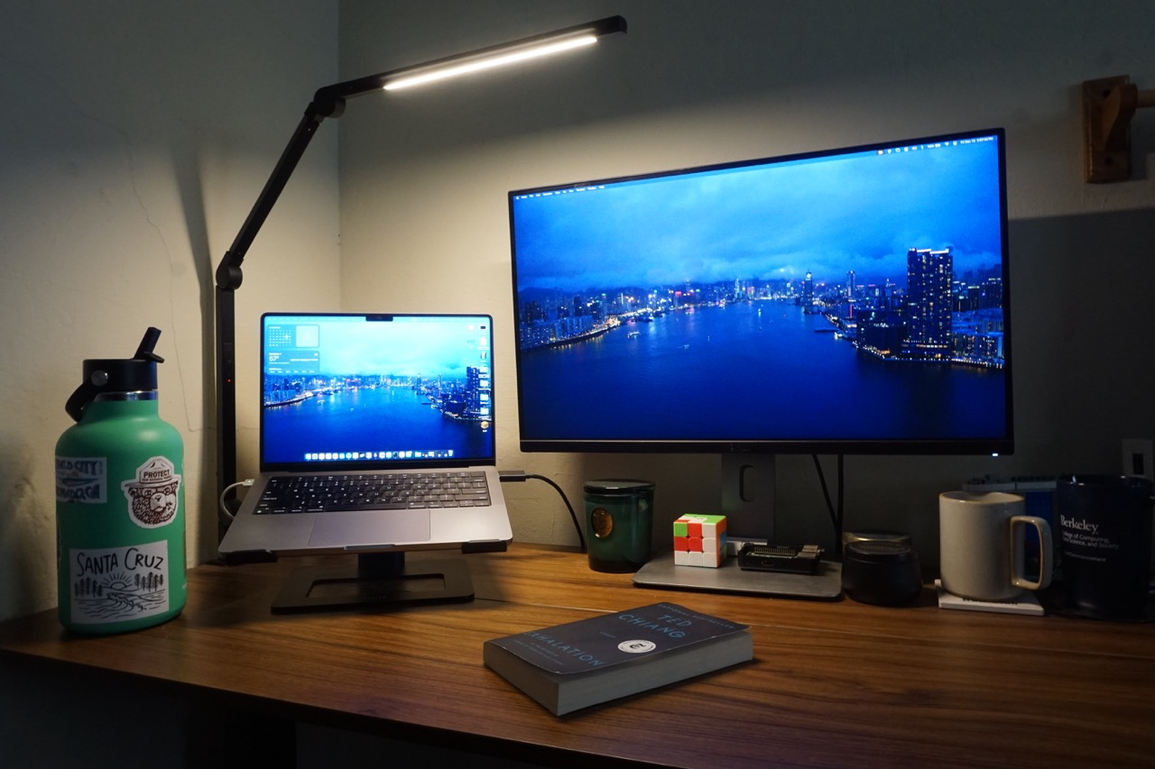
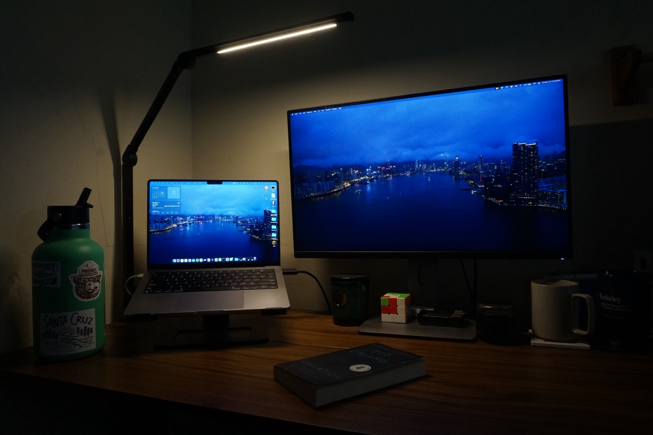
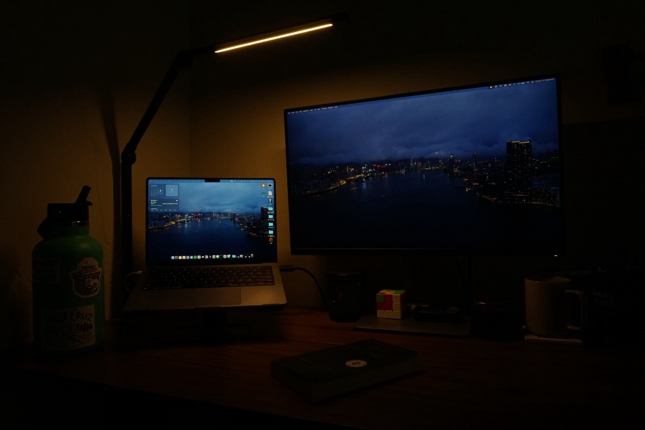
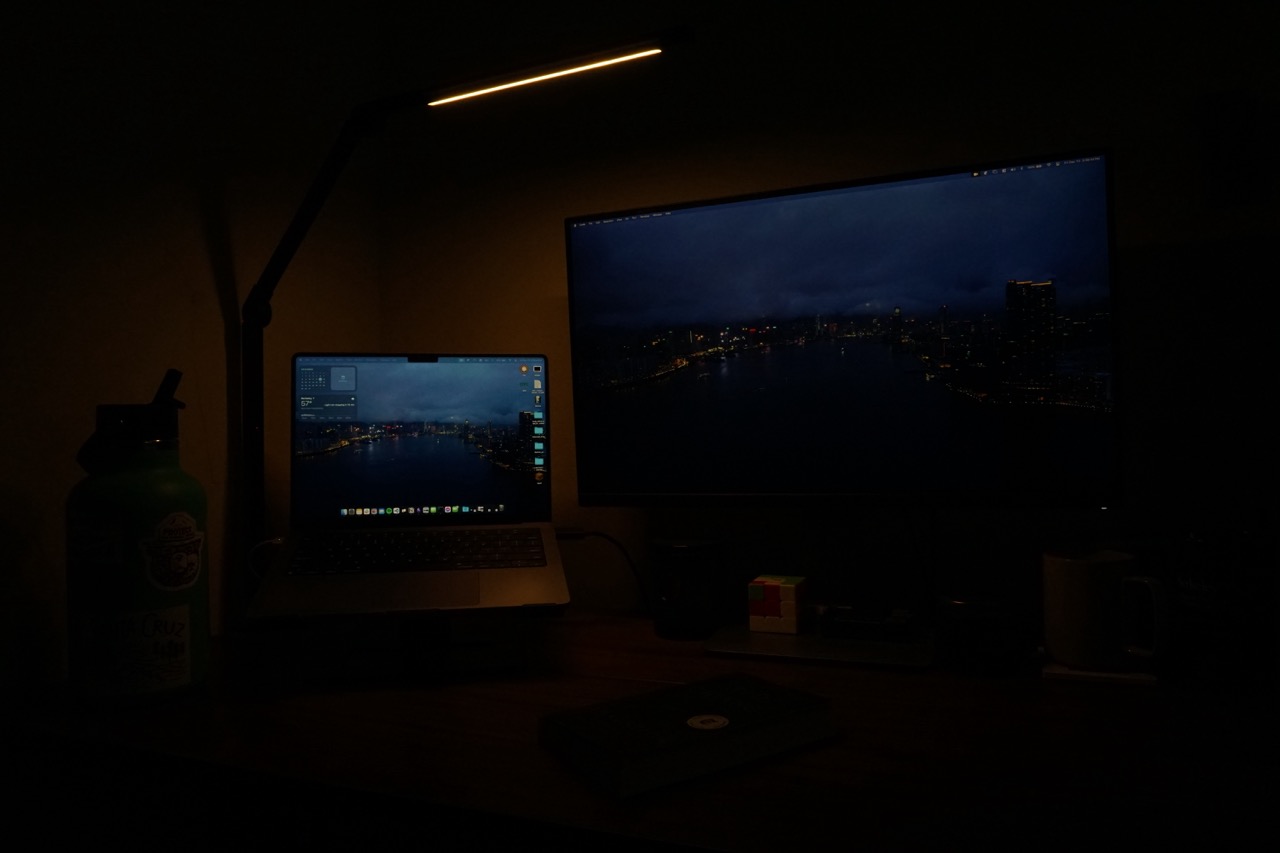
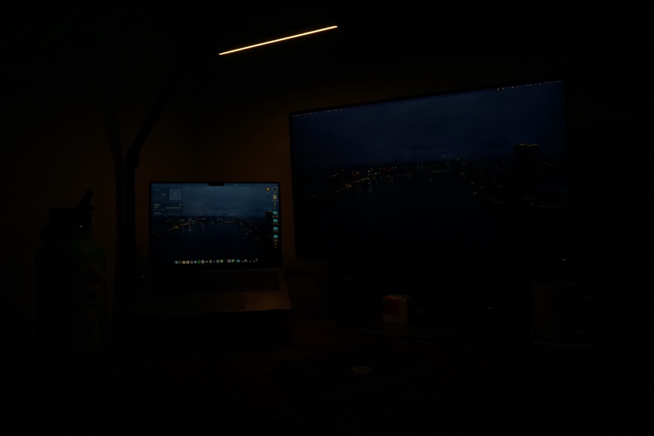
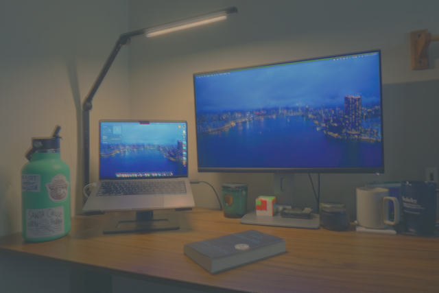
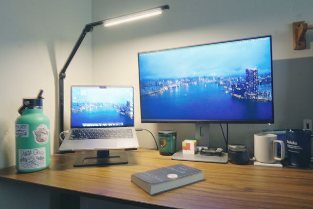
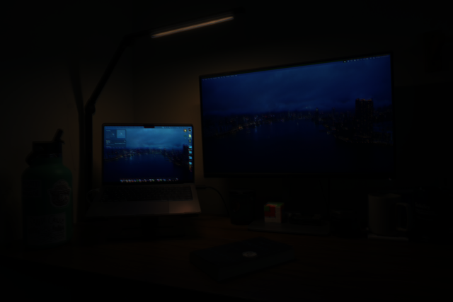
Bells and Whistles!

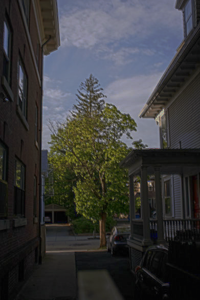
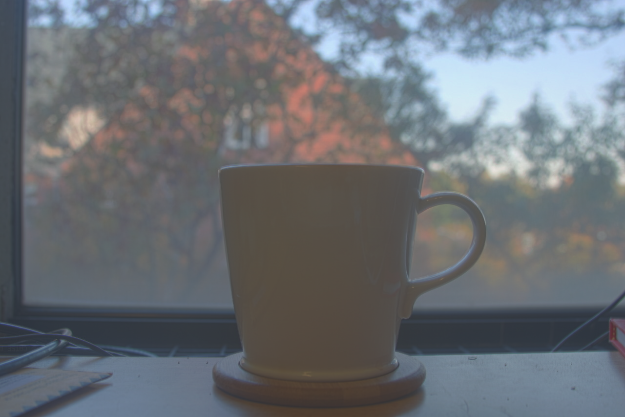
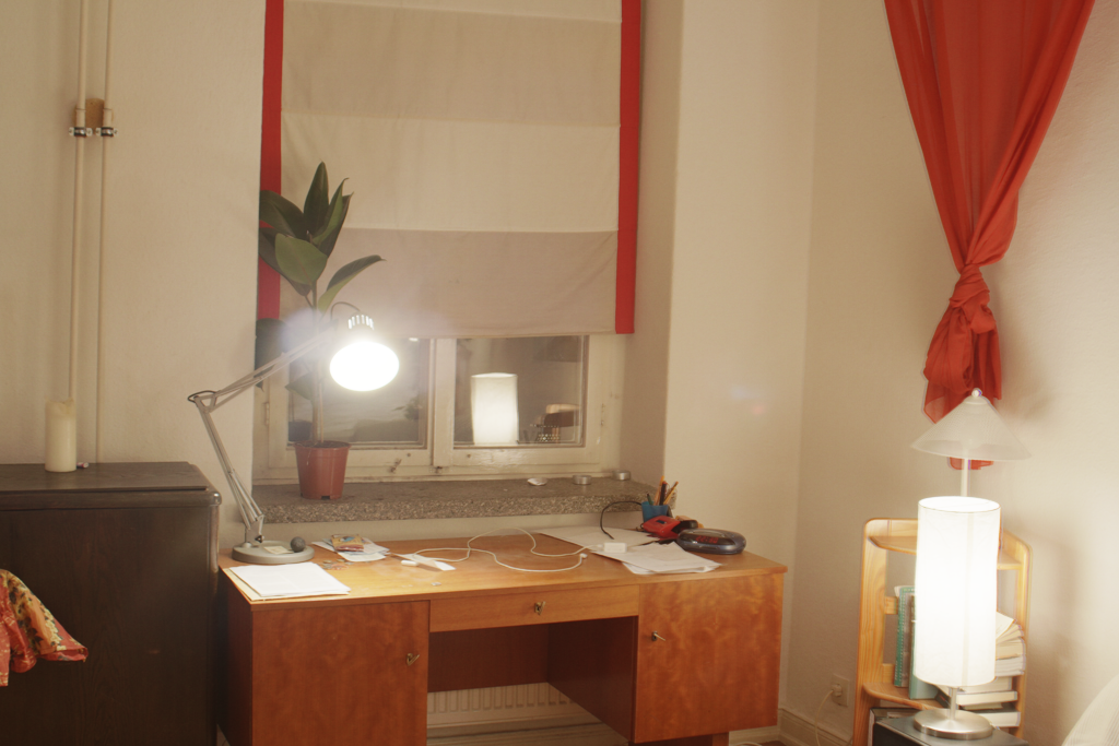
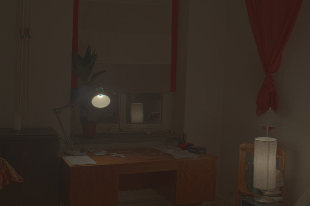
For my bells and whistles I used my own images and ran them through the HDR implementation. I used a set of images of my desk and stacked some boxes to create a stationary place to put my camera. I captured 6 frames with varying exposures. Although I think I still slightly moved the camera between shots while I was changing the exposure. Below are my results.

Conclusion

I enjoyed working on these projects, I particularily liked the AR project as I thought the final output was very fascinating and being able to work with videos was also a first for me. I also enjoyed the HDR project as it gave me more practice with reading research papers and I found the results to be very pretty. The Durand output produced a cool tone in my opinion and I learned a lot about how to manipulate images to produce a better result.